tecznotes
Michal Migurski's notebook, listening post, and soapbox. Subscribe to ![]() this blog.
Check out the rest of my site as well.
this blog.
Check out the rest of my site as well.
Dec 31, 2012 2:01am
back to webgl and nokia’s maps
I’m picking up last year’s data format exploration and dusting it off some to think about WebGL shader programming. More on this later. Click through to interactive demos below, if your browser speaks ArrayBuffer and WebGL. Tested with Chrome.


Dec 14, 2012 6:58am
three ways fastly is awesome
We released the Google #freeandopen project earlier this month.
In a few days the International Telecommunication Union, a UN body made up of governments around the world, will be meeting in Qatar to re-negotiate International Telecommunications Regulations. These meetings will be held in private and behind closed doors, which many feel runs counter to the open nature of the internet. In response to this, Google is asking people to add their voice in favor of a free and open internet. Those voices are being displayed, in as close to real time as we can manage, on an interactive map of the world, designed and built by Enso, Blue State Digital, and us!
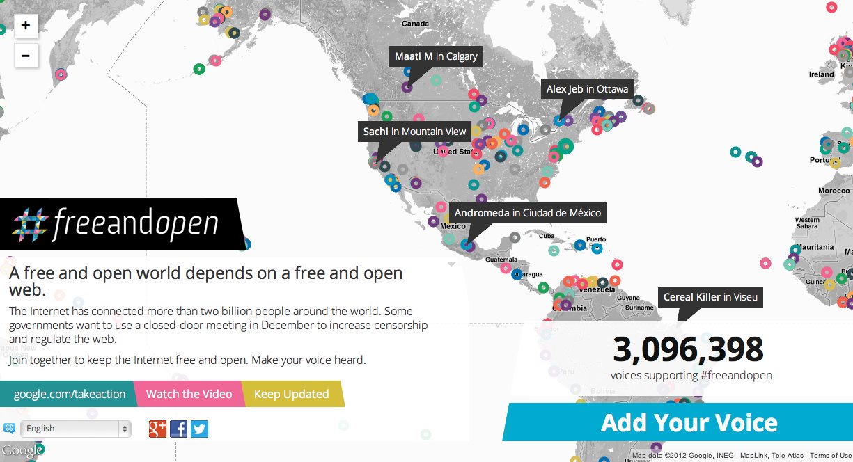
It was a highly-visible and well-trafficked project, linked directly from Google’s homepage for a few days, and we ultimately got over three million direct engagements in and amongst terabytes of hits and visits. We built it with a few interesting constraints: no AWS, rigorous Google security reviews, and no domain name until very late in the process. We would typically use Amazon’s services for this kind of thing, so it was a fun experiment to determine the mix of technology providers we should use to meet the need. Artur Bergman and Simon Wistow’s edge cache service Fastly stood out in particular and will probably be a replacement for Amazon Cloudfront for me in the future.
Fastly kicked ass for us in three ways:
First and easiest, it’s a drop-in replacement for Cloudfront with a comparable billing model. For some of our media clients, we use existing corporate Akamai accounts to divert load from origin servers. Akamai is fantastic, but their bread and butter looks to be enterprise-style customers. It often takes several attempts to communicate clearly that we want a “dumb” caching layer, respecting origin server HTTP Expires and Cache-Control headers. Fastly uses a request-based billing model, like Amazon, so you pay for the bandwidth and requests that you actually use. Bills go up, bills go down. The test account I set up back when I was first testing Fastly worked perfectly, and kept up with demand and more than a few quick configuration chanages.
Second, Fastly lets you modify with response headers. It’s taken Amazon S3 three years to release CORS support, something that Mike Bostock and I were asking them about back when we were looking for a sane way to host Polymaps example data several years ago (we ended up using AppEngine, and now the example data is 410 Gone). Fastly has a reasonably-simple UI for editing configurations, and it’s possible to add new headers to responses under “Content,” like this:
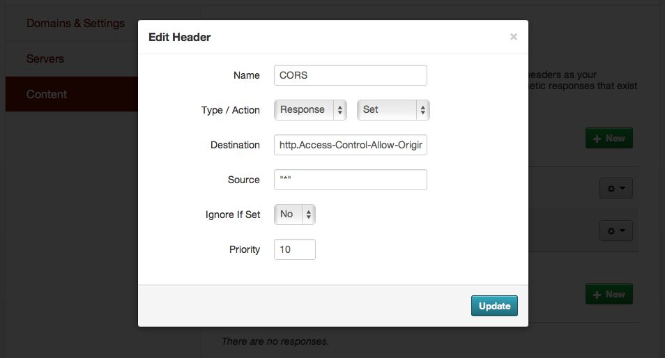
Now we could skip the JSONP dance and use Ajax like JJG intended, even though the source data was hosted on Google Cloud Storage where I couldn’t be bothered to figure out how to configure CORS support.
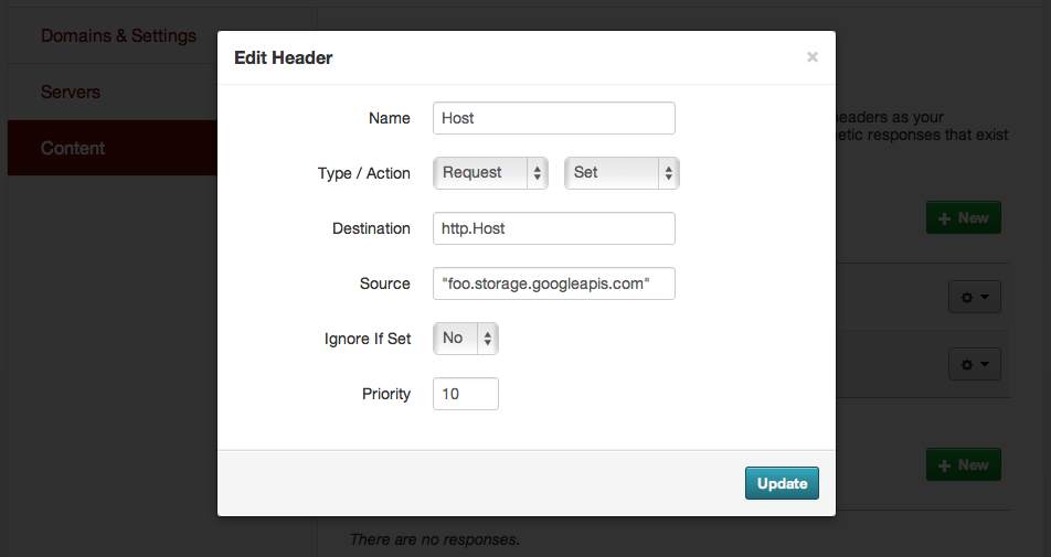
Finally, you can perform some of these same HTTP army knife magic on the request headers to the origin server. I’m particularly happy with this trick. Both Google Cloud Storage and Amazon S3 allow you to name buckets after domains and then serve from them directly with a small amount of DNS magic, but neither appears to allow you to rename a bucket or easily move objects between buckets, so you would need to know your domain name ahead of time. In the case of GCS, there’s an additional constraint that requires you to prove ownership of a domain name before the service will even let you name a bucket with a matching name. We had to make our DNS changes in exactly one move at a point in the project where a few details remained unclear, so instead of relying on DNS CNAME/bucket-name support we pointed the entire subdomain to Fastly and then did our configuration there. We were able to keep our original bucket name by rewriting the HTTP Host header on each request, in effect lying to the storage service about the requests it was seeing so we could defer our domain changes until later:
It sounds small, but on a very fast-moving project with a lot of moving pieces and a big client to keep happy, I was grateful for every additional bit of flexibility I could find. HTTP offers so many possibilities like this, and I love finding ways to take advantage of the distributed nature of the protocol in support of projects for clients much, much larger than we are.

Dec 8, 2012 10:58pm
fourteen years of pantone colors-of-the-year
I love the language patterns in press releases that accompany annual announcements, like Pantone’s Color Of The Year. Leatrice Eiseman, executive director of the Pantone Color Institute, has been providing adjectives and free-associating since 1999. Between 9/11 and the economy, a lot of political freight gets bundled into these packages as well—“concern about the economy” is first mentioned in late 2005 (sand dollar).

That’s the news if you were waiting to plan any decorating updates around Pantone’s Color of the Year announcement.
“Green is the most abundant hue in nature—the human eye sees more green than any other color in the spectrum,” says Leatrice Eiseman, executive director of the Pantone Color Institute. “Symbolically, Emerald brings a sense of clarity, renewal and rejuvenation, which is so important in today’s complex world.”
Emerald green, being associated with gemstone for which it is named, is a sophisticated and luxurious choice, according to Eiseman. “It’s also the color of growth, renewal and prosperity—no other color conveys regeneration more than green. For centuries, many countries have chosen green to represent healing and unity.”

The 2011 color of the year, PANTONE 18-2120 Honeysuckle, encouraged us to face everyday troubles with verve and vigor. Tangerine Tango, a spirited reddish orange, continues to provide the energy boost we need to recharge and move forward.
“Sophisticated but at the same time dramatic and seductive, Tangerine Tango is an orange with a lot of depth to it,” said Leatrice Eiseman, executive director of the Pantone Color Institute®. “Reminiscent of the radiant shadings of a sunset, Tangerine Tango marries the vivaciousness and adrenaline rush of red with the friendliness and warmth of yellow, to form a high-visibility, magnetic hue that emanates heat and energy.”

Honeysuckle is encouraging and uplifting. It elevates our psyche beyond escape, instilling the confidence, courage and spirit to meet the exhaustive challenges that have become part of everyday life.
“In times of stress, we need something to lift our spirits. Honeysuckle is a captivating, stimulating color that gets the adrenaline going—perfect to ward off the blues,” explains Leatrice Eiseman, executive director of the Pantone Color Institute®. “Honeysuckle derives its positive qualities from a powerful bond to its mother color red, the most physical, viscerally alive hue in the spectrum.”

Combining the serene qualities of blue and the invigorating aspects of green, Turquoise evokes thoughts of soothing, tropical waters and a languorous, effective escape from the everyday troubles of the world, while at the same time restoring our sense of wellbeing.
“In many cultures, Turquoise occupies a very special position in the world of color,” explains Leatrice Eiseman, executive director of the Pantone Color Institute®. “It is believed to be a protective talisman, a color of deep compassion and healing, and a color of faith and truth, inspired by water and sky. Through years of color word-association studies, we also find that Turquoise represents an escape to many—taking them to a tropical paradise that is pleasant and inviting, even if only a fantasy.”

In a time of economic uncertainty and political change, optimism is paramount and no other color expresses hope and reassurance more than yellow. “The color yellow exemplifies the warmth and nurturing quality of the sun, properties we as humans are naturally drawn to for reassurance,” explains Leatrice Eiseman, executive director of the Pantone Color Institute®. “Mimosa also speaks to enlightenment, as it is a hue that sparks imagination and innovation.”

Combining the stable and calming aspects of blue with the mystical and spiritual qualities of purple, Blue Iris satisfies the need for reassurance in a complex world, while adding a hint of mystery and excitement.
“From a color forecasting perspective, we have chosen PANTONE 18-3943 Blue Iris as the color of the year, as it best represents color direction in 2008 for fashion, cosmetics and home products,” explains Leatrice Eiseman, executive director of the Pantone Color Institute®. “As a reflection of the times, Blue Iris brings together the dependable aspect of blue, underscored by a strong, soul-searching purple cast. Emotionally, it is anchoring and meditative with a touch of magic. Look for it artfully combined with deeper plums, red-browns, yellow-greens, grapes and grays.”

In a time when personality is reflected in everything from a cell phone to a Web page on a social networking site, Chili Pepper connotes an outgoing, confident, design-savvy attitude.
“Whether expressing danger, celebration, love or passion, red will not be ignored,” explains Leatrice Eiseman, executive director of the Pantone Color Institute®. “In 2007, there is an awareness of the melding of diverse cultural influences, and Chili Pepper is a reflection of exotic tastes both on the tongue and to the eye. Nothing reflects the spirit of adventure more than the color red. At the same time, Chili Pepper speaks to a certain level of confidence and taste. Incorporating this color into your wardrobe and living space adds drama and excitement, as it stimulates the senses.”
“In 2007, we’re going to see people making greater strides toward expressing their individuality,” says Lisa Herbert, executive vice president of the fashion, home and interiors division at Pantone.

Pantone’s Sand Dollar 13-1106 was the 2006 Color of the Year. It’s considered a neutral color that expresses concern about the economy.

Pantone’s Blue Turquoise 15-5217 was the 2005 Color of the Year. Following the theme of nature from 2004’s color, Tiger Lily, Blue Turquoise is the color of the sea and is also used in tapestries and other artworks from the American Southwest.

Pantone’s Tiger Lily 17-1456 was the 2004 Color of the Year. It acknowledges the hipness of orange, with a touch of exoticism.
With inspiration from the natural flower, this warm oragne contains the very different red and yellow. One of these colors evokes power and passion while the other is hopeful. This combination creates a bold and rejuvinating color.

Pantone’s Aqua Sky 14-4811 was the 2003 Color of the Year. A cool blue was chosen in hopes to restore hope and serenity. This quiet blue is more calming and cool than other blue-greens.

The color was chosen in recognition of the impact of September 11 attacks. This red is a deep shade and is a meaningful and patriotic hue. Red is known as a color of power and/or passion and is thus associated with love.


This color represents the millennium because of the calming zen state of mind it induces. Blue is known to be a calming color.
Leatrice Eiseman, executive director of the Pantone Color Institute®, said that looking at a blue sky brings a sense of peace and tranquility. “Surrounding yourself with Cerulean blue could bring on a certain peace because it reminds you of time spent outdoors, on a beach, near the water—associations with restful, peaceful, relaxing times. In addition, it makes the unknown a little less frightening because the sky, which is a presence in our lives every day, is a constant and is always there,” Eiseman said.
Nov 29, 2012 7:37am
gamma shapes for obama
Back in April, I bailed to Chicago for a week to volunteer with the Obama campaign tech team. It’s the team you’ve read all about, the one CTO’d by Harper Reed that blew the doors off the Romney campaign, and I was unbelievably lucky to spend one too-short week seven months ago working with the group right in their office.
Interestingly, what I ended up working on was a direct descendant of the precinct geometries that Marc Pfister mentioned in the comments of my old post:
We were manually fixing precinct data. We’d look at address-level registration data and rebuild precincts from blocks. A lot of it could probably have been done with something like Clustr and some autocorrelation. But basically you would look at a bunch of points and pick out the polygons they covered.
Clustr is a tool developed by Schuyler Erle and immortalized by Aaron Cope’s work on Flickr alpha shapes:
For every geotagged photo we store up to six Where On Earth (WOE) IDs. … Over time this got us wondering: If we plotted all the geotagged photos associated with a particular WOE ID, would we have enough data to generate a mostly accurate contour of that place? Not a perfect representation, perhaps, but something more fine-grained than a bounding box. It turns out we can.
Schuyler followed up on the alpha shapes project with beta shapes, a project used at SimpleGeo to correlate OSM-based geometry with point-based data from other sources like Foursquare or Flickr, generating neighborhood boundaries that match streets through a process of simple votes from users of social services. For campaign use, up-to-date boundaries for legislative precincts remains something of a holy grail. We would need an evolution of alpha- and beta-shapes that I’m going to go ahead and call “gamma shapes”.
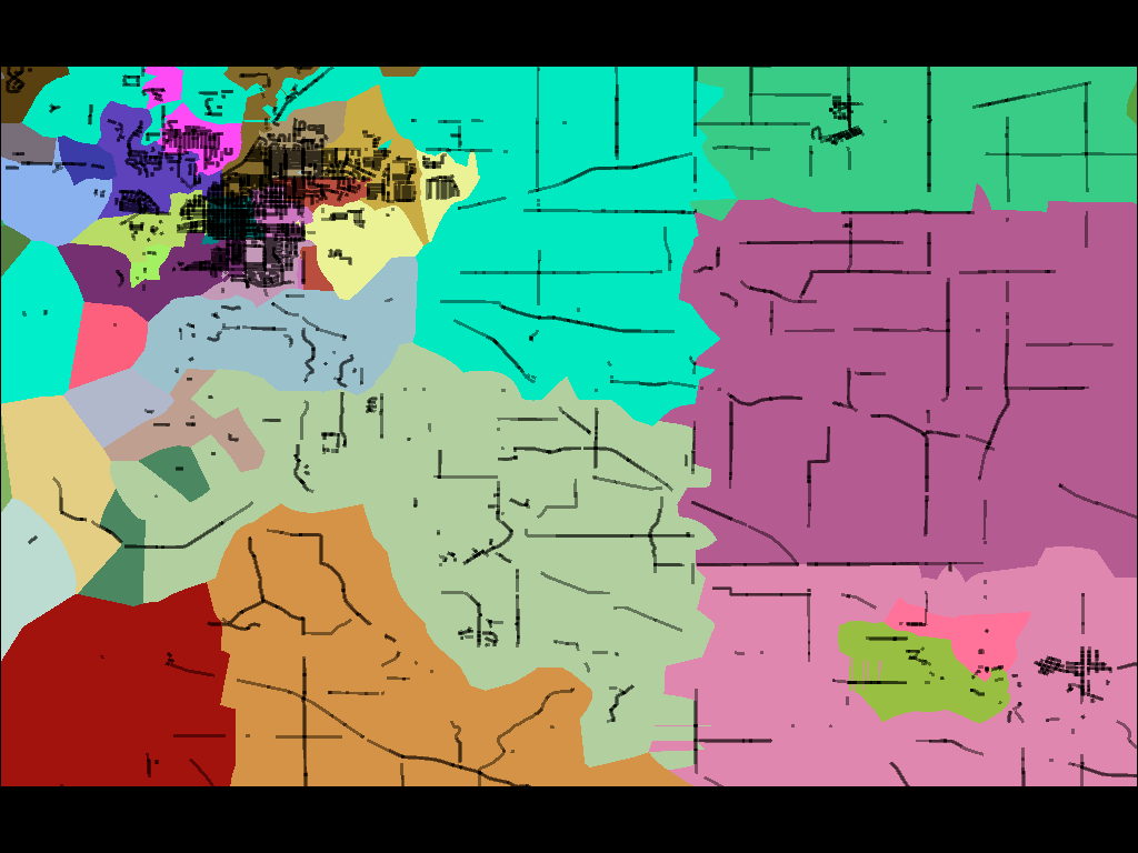
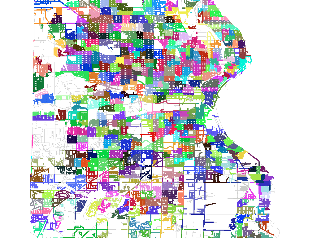
Gamma shapes are defined by information from the Voter Information Project, which provides data from secretaries of state who define voting precincts prior to election day. While data providers like the U.S. Census provide clean shapefiles for nationwide districts, these typically lag the official definitions by many months, and those official definitions are in notable flux in the immediate lead-up to a national election. Everything was changing, and we needed a picture like this to accurately help field offices before November 6:
Unlike Flickr and SimpleGeo’s needs, precinct outlines are unambiguous and non-overlapping. It’s not enough to guess at a smoothed boundary or make a soft judgement call. As Anthea Watson-Strong and Paul Smith showed me, legislative precincts are defined in terms of address lists, and if your block is entirely within precinct A except for one house that’s in B, that’s an anomaly that must be accounted for in the map, such as this district with a weird, non-contiguous island:
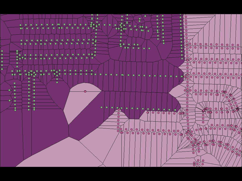
The shapes above should look familiar to you if you’ve ever seen the Voronoi diagram, one of this year’s smoking-hot fashion algorithms.

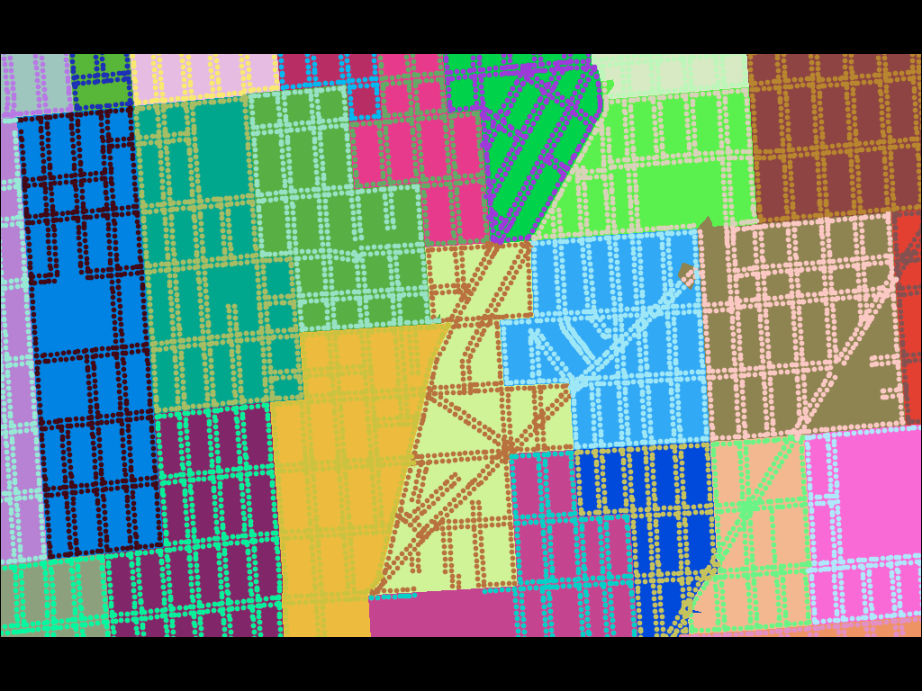
When you remove the clipping boundaries defined by TIGER/Line, you reveal a simple Voronoi tessellation of our original precinct-defining address points, each one with a surrounding cell of influence that shows where that precinct begins and ends. Voronoi allows us to define a continuous space based on distance to known points, and establishes cut lines that we can use to subdivide a TIGER-bounded block into two or more precincts. In most cases it’s not needed, because precinct boundaries are generally good about following obvious lines like roads or rivers. Sometimes, for example in cases of sparse road networks outside towns or demographic weirdness or even gerrymandering, the Voronoi are necessary.
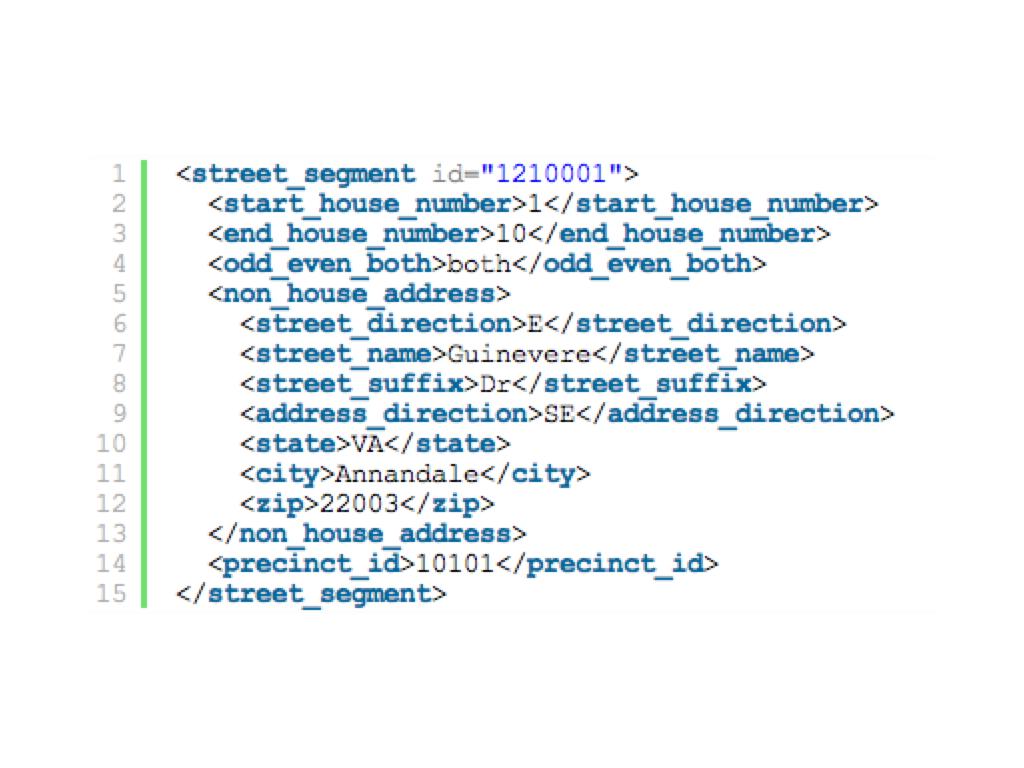
The points in some of the images below are meant to represent individual address points (houses), but for most states precincts are defined in terms of address ranges. For example, the address numbers 100 through 180 on the even side of a street might be one precinct, while numbers 182 though 198 are another. In these case, I’m using TIGER/Line and Postgis 2.0’s new curve offset features to fake a line of houses by simply offsetting the road in either direction and clipping it to a range.
For a large city, such as this image of Milwaukee, there can be hundreds of precincts each just a few blocks in size:
In the end, the Voter Information Project source data ended up being of insufficient quality to support an accurate mapping operation, so this work will need to continue at some future date with new fresh data. Precincts change constantly, so I would expect to revisit this as a process rather than an end-product. Sadly, much of the code behind this project is not mine to share, so I can’t simply open up a repository as I normally would. Next time!

Nov 26, 2012 7:13am
teasing out the data
I spoke in New York two weeks ago, about the shyness of good data and the process of surfacing it to new audiences. I did two talks, one for the Visualized conference and the second for James Bridle’s New Aesthetic class at NYU’s Interactive Telecommunications Program.

In February 2010, The Economist published its special report on “the data deluge,” covering the emergence and handling of big data. At Stamen, we’ve long talked about our work as a response to everything informationalizing, the small interactions of everyday lives turning into gettable, mineable, patternable strands of digital data. At Visualized, at least two speakers described the bigness of data and explicitly referenced the 2010 Economist cover for support. I’ve been trying to get a look at the flip side of this issue, thinking about the use of small data and the task of daylighting tiny streams of previously-culverted information.

Aaron Cope joked about the concept of informationalized-everything as sensors gonna sense, the inevitability of data streams from receivers and robots placed to collect and relay it. I recently spent a week in Portland, where I met up with Charlie Loyd whose data explorations of MODIS satellite imagery arrested my attention a few months ago. Charlie has been treating MODIS’s medium-resolution imagery as a temporal data source, looking in particular at the results of NASA’s daily Arctic mosaic. Each day’s 1km resolution polar projection shows the current state of sea ice and weather in the arctic circle, and Loyd’s yearlong averages of the data show ghostly wisps of advancing and retreating ice floes and macro weather patterns. The combined imagery is pale and paraffin-like, a combination of Matthew Barney and Edward Imhof. I’m drawn to the smooth grayness and through Loyd’s painstaking numeric experimentation with the data I remember the tremendous difficulty of drawing data from a source like MODIS. Nevermind the need to convert the blurry-edged image swaths, collected on a constant basis from 99-minute loops around the earth by MODIS’s Aqua and Terra hardware, the downstream use of the data by researchers at Boston University in 2006 to derive a worldwide landcover dataset is an example of interpretative effort. The judgements of B.U. classifiers are tested by spot checks in the United States, visits to grid squares to determine that there are indeed trees or concrete there. The alternative 2009 GLOBCOVER dataset offers a different interpretation of some of the same areas, influenced by the European location of the GLOBCOVER researchers and the check locations available to them. Two data sets, two sets of researchers, two interpretations governed by available facts, two sets of caveats to keep in mind when using the data.
Civic-scale data offers some of the same opportunities for interpretive difficulty. For years I’ve been interested in the movements of private Silicon Valley corporate shuttles, and thanks to the San Jose Zero1 Biennial we’ve been able to support that fascination with actual data.

At Visualized, I explored the idea of good data as “shy data,” looking at the work we did in 2006/2007 on Crimespotting and our more-recent work on private buses. The city of San Francisco had already studied the role of shuttle services in San Francisco, yet the report was not sparking the kind of dialogue these new systems need. Oakland was already publishing crime data, but it wasn’t seeing the kinds of day-to-day use and attention that it needed.

Exposing data that’s shy or hidden is often just introducing it to a new audience, whether that’s The New York Times looking at Netflix queues or economists getting down in the gutters and physically measuring cigarette butt lengths to measure levels of poverty and deprivation.
The Economist-style “data deluge” metaphor is legitimate, but seems somehow less cuspy than completely new kinds of data just peeking out for the first time. The deluge is about operationalized, industrialized streams. What are the right approaches for teasing something out that’s not been seen before, or not turned into a shareable form?
Oct 29, 2012 7:15am
the city from the valley: shuttle project for zero1
Last weekend, I participating in a panel on data and citizen sensors for the Urban Prototyping Festival. Our moderator was Peter Hirshberg, with co-panelists Sha Hwang, Genevieve Hoffman, Shannon Spanhake and Jeff Risom:
Urban Insights: Learning about Cities from Data & Citizen Sensors. Collection and visualization of urban data have quickly become powerful tools for municipal governance. Citizens now have the capacity to act as sensors, data analysts, information designers, or all of the above to help cities better understand themselves. This panel will focus on the evolving role of open data and its applications to the public sector.
In thinking about how to talk about data collection, I wanted to highlight a recent project that we at Stamen did for the Zero1 festival in San Jose, The City from the Valley: “An alternate transportation network of private buses—fully equipped with wifi—thus threads daily through San Francisco, picking up workers at unmarked bus stops (though many coexist in digital space), carrying them southward via the commuter lanes of the 101 and 280 freeways, and eventually delivers them to their campuses.”
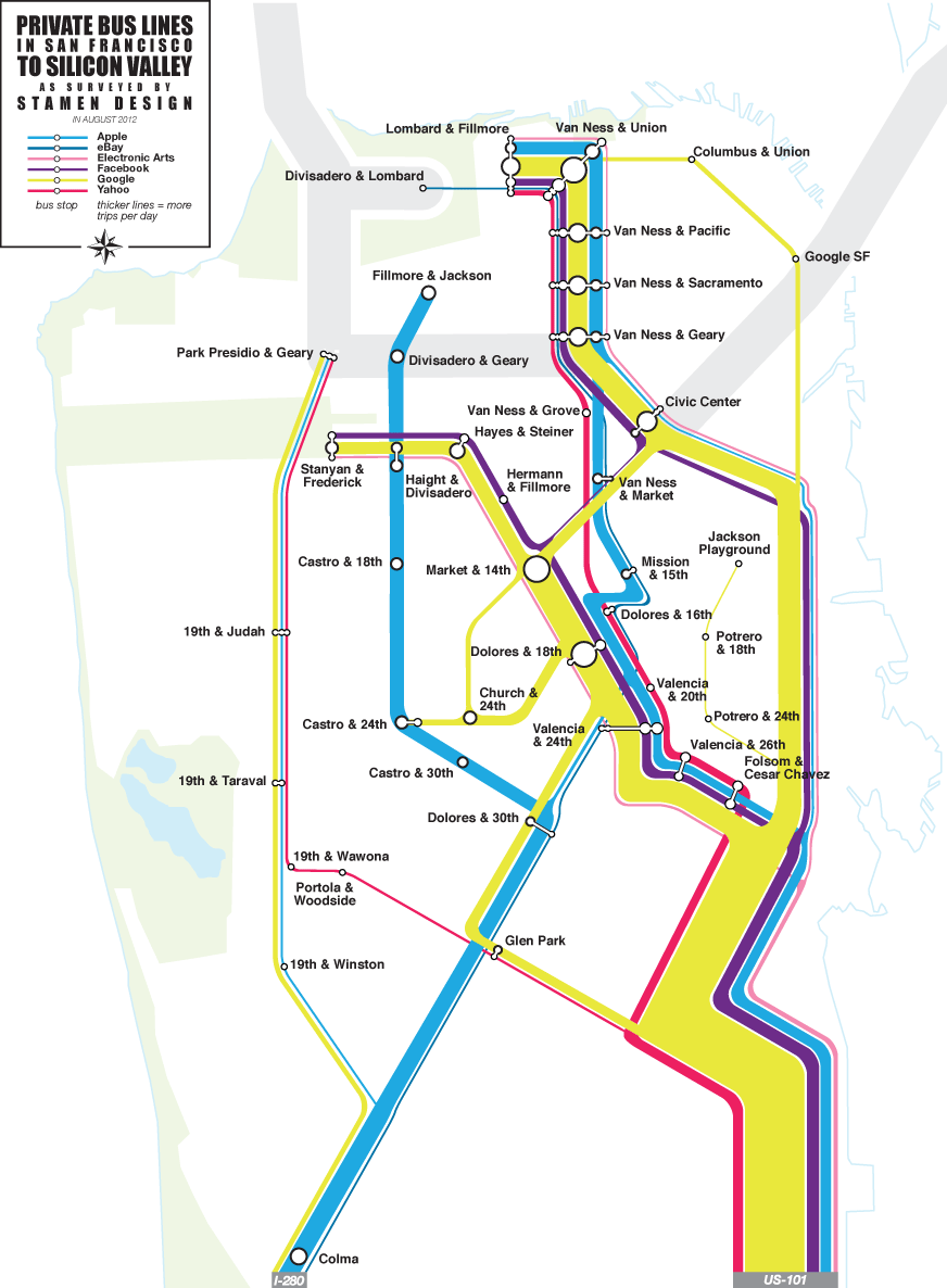
I’ve been fascinated by these buses for a few years now, first realizing the extent of the network over periodic Mission breakfast with Aaron. We’d drink our coffee and watch one after another after another gleaming white shuttle bus make its way up Valencia. I’d hear from friends about how the presence of the shuttles was driving SF real estate prices, and as a longtime Mission district weekday occupant the change in the local business ecology is unmissable.
The results of our observations suggest that this network of private shuttles carries about 1/3rd of Caltrain’s ridership every day, a huge number. I’m not sure myself of the best way to look at it. It’s clearly better to have people on transit instead of personal cars, but have we accidentally turned San Francisco into a bedroom community for the south bay instead?
According to a survey by the San Francisco County Transportation Authority, 80 percent of people riding the shuttles said they would be driving to work or otherwise wouldn't be able to live in San Francisco if they couldn't get the company-sponsored rides to work. —SF Supervisor Proposes Strict Regulations For Corporate Shuttles.
What of the Mission district, whose transformation into an artisinal brunch wonderland I’ve found aesthetically challenging? Maybe more significantly, what of the private perks offered by valley companies, of which private transport is just one? I think Google, Facebook, Apple and others have all done their own math and determined that it’s advantageous to move, feed, clothe, and generally coddle your workforce. This math scales a lot more than is obvious, and as a country we should be looking at things like the Affordable Care Act in a more favorable light, perhaps asking companies who need to move employees up and down the peninsula to pay more into Caltrain instead of running their own fleets. Election time is near, and even though my mind is made up the public vs. private debate in this country remains wide open. Am I comfortable with a Bay Area where the best-paid workers are also subject to a distorted view of reality, having their most basic needs passively met while those not lucky enough to work in the search ad mines have to seek out everything for themselves? Privilege is driving a smooth road and not even knowing it.
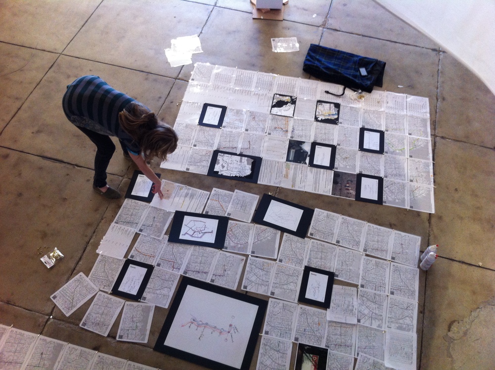
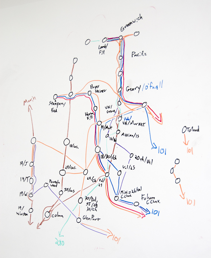
This fascination, by the way, is my total contribution to the project—once we all decided that the buses were worth exploring and after Eric, George and I had spent a morning counting them from the corner of 18th & Dolores to make sure we weren’t crazy, the gears of the studio kicked in and the project was born. Nathaniel and Julie worked with local couriers to track sample routes, and we used Field Papers to note passenger counts and stops. Zach looked at Foursquare checkins for clues. Nathaniel and Zach created the flow map above to illustrate our guesses at ridership and routes, and the whole thing went up in San Jose last month:
Oct 7, 2012 6:50pm
openstreetmap in postgres
I was chatting with Sha this weekend about how to get data out of OpenStreetMap and into a database, and realized that it’s possible no one’s really explained a full range of current options in the past few years. Like a lot of things with OSM, information about this topic is plentiful but rarely collected in one place, and often consists of half-tested theories, rumors, and trace amounts of accurate fact based on personal experience earned in a hurry while at the point of loaded yak.
At first glance, OSM data and Postgres (specifically PostGIS) seem like a natural, easy fit for one another: OSM is vector data, PostGIS stores vector data. OSM has usernames and dates-modified, PostGIS has columns for storing those things in tables. OSM is a worldwide dataset, PostGIS has fast spatial indexes to get to the part you want. When you get to OSM’s free-form tags, though, the row/column model of Postgres stops making sense and you start to reach for linking tables or advanced features like hstore.
There are three basic tools for working with OSM data, and they fall along a continuum from raw data on one end to render-ready map linework on the other.
Osmosis
Osmosis is the granddaddy of OpenStreetMap tools:
The tool consists of a series of pluggable components that can be chained together to perform a larger operation. For example, it has components for reading from database and from file, components for writing to database and to file, components for deriving and applying change sets to data sources, components for sorting data, etc.
Mostly Osmosis is used to retrieve full planet dumps or local extracts of OSM data and convert it to various formats, strip it of certain features, or merge multiple parts together. Osmosis can write to Postgres using a snapshot schema, with nodes stored as real PostGIS point geometries and ways optionally stored as Linestrings. OSM tags are stored in hstore columns as key/value mappings. User information goes into a separate table.
The Osmosis snapshot schema is great if you want:
- Original nodes and you don’t care what streets they’re a part of.
- Metadata about OSM such as owners of particular ways.
- Downstream extracts from your database.
Snapshot schema tables: nodes (geometry), ways (optional geometry), relation_members, relations, schema_info, users, way_nodes.
I’m fairly new to Osmosis myself, just starting to get my head around its pitfalls.
Osm2pgsql
Osm2pgsql is in common use for cartography, “often used to render OSM data visually using Mapnik, as Mapnik can query PostgreSQL for map data.” Osm2pgsql is lossy, and you can tweak its terribly-named “style file” to decide which original tags you want to keep for rendering. Tags are converted into Postgres column names, with newer versions of Osm2pgsql also supporting the use of hstore to save complete tag sets. Data ends up in three main tables, grouped into points, lines and polygons.
Osm2pgsql will get you:
- An easy, no-configuration direct import organized by geometry type.
- Reasonably fast selections and renders by Mapnik.
- Automatic spherical mercator projection.
- A list of affected tiles if you use it on a changeset.
I’ve never successfully run Osm2pgsql without using the “slim” option, which stores additional data in Postgres and makes it possible apply changes later. Osm2pgsql tables: point (geometry), line (geometry), polygon (geometry), nodes (data), rels (data), ways (data), roads (never used this one).
I’ve included ready-to-use shapefiles of Osm2pgsql data in the Metro Extracts.
Imposm
Imposm is at the far end of the scale, producing topic-specific tables that you define.
Imposm is an importer for OpenStreetMap data. It reads XML and PBF files and can import the data into PostgreSQL/PostGIS databases. It is designed to create databases that are optimized for rendering/WMS services.
Where Osm2pgsql gets you a single table for all linestrings, Imposm can give you a table for roads, another for rail, a third for transit points, and so on. It does this by using a mapping file written in Python which selects groups of tags to map to individual tables. Imposm can perform a ton of upfront work to make your downstream Mapnik rendering go faster, and requires significantly more data preparation effort if you want to depart from default schemas. I’ve been working on an all-purpose mapping based on High Road just to make this easier. The cost of upfront work is tempered somewhat by Imposm’s use of concurrency and its separation of database population from deployment, something you normally do manually in Osm2pgsql.
Imposm is great for:
- Faster, smaller, more render-ready data.
- Automatic simplified geometry tables.
Use it if you’re working on cartography and already know how you want to map OSM data. I’ve had good experiences using Osm2pgsql together with Imposm, building up complex queries from generic Osm2pgsql data and then translating them into Imposm mappings. I’ve also been using it to perform street name abbreviations at import time, greatly improving the visual quality of road names in final maps.
Sample tables from my own mapping: green_areas, places, buildings, water_areas, roads and rails divided up by zoom level.
I’ve included ready-to-use shapefiles of Imposm data in the Metro Extracts.
Takeaway
Use Osmosis if you’re interested in data. Start with Osm2pgsql if you want to render maps. Move to Imposm once you know exactly what you want.
Oct 7, 2012 7:36am
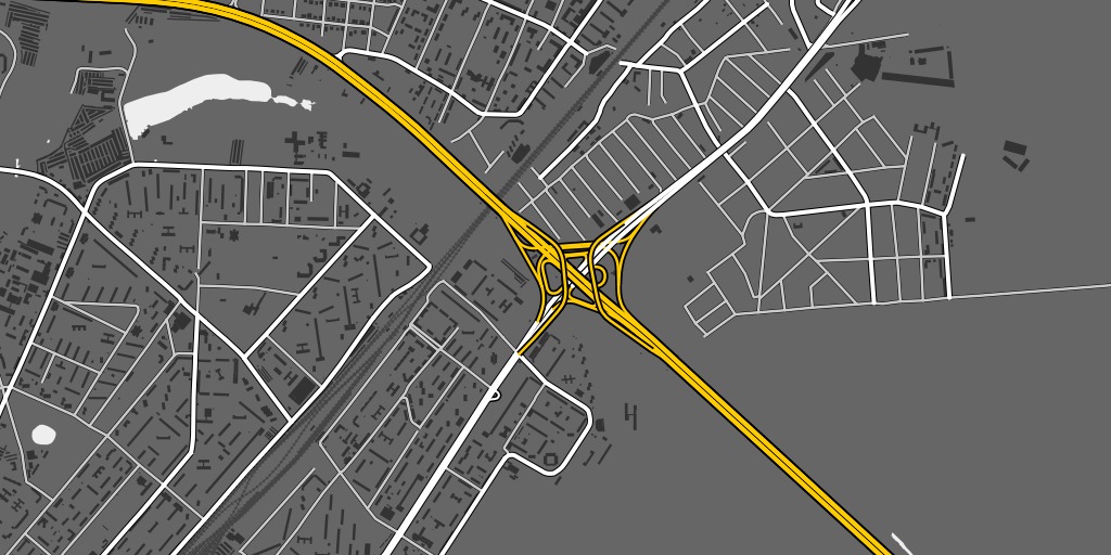
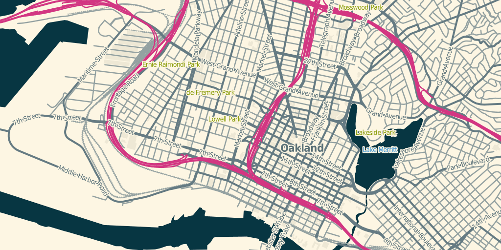
maps of lake merritt
Lake Merritt might be the Lenna of online cartography samples. Only one of these comes from someone who actually lives in Oakland:
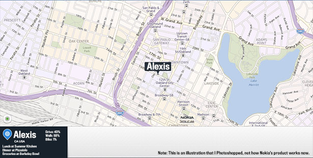
—Alexis Madrigal in The Atlantic, The Forgotten Mapmaker.
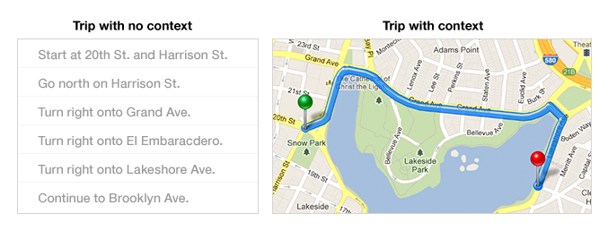
—Bret Victor on Learnable Programming.
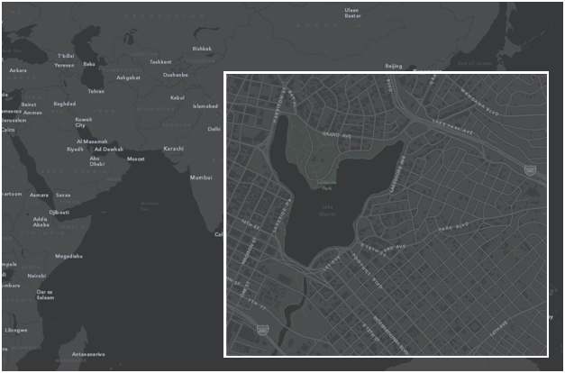
—Mamata Akella on Esri Canvas Maps.
Sep 26, 2012 5:49am
538 with 42 to go
Day-by-day for the past three weeks, just the parts of Nate Silver’s 538 state-by-state probabilities map that change in 8x8 pixel blocks.
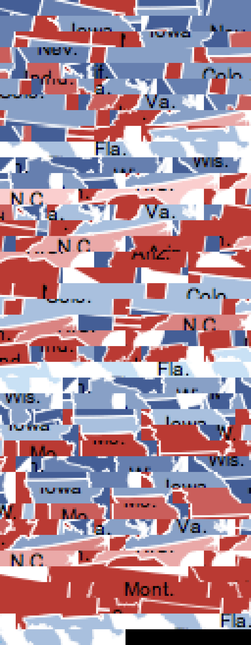
For the wha, see also the iPhone 5 website teardown.
Sep 18, 2012 6:35am
a beginners guide to streamed data from Twitter
A few months ago, Shawn Allen and I taught a class on visualizing and mapping data at GAFFTA. We covered everything from client-side Javascript map interaction, basemap design with OpenStreetMap and Mapnik, dynamic in-browser graphics with D3, to ingesting and handling raw open public data. For one set of exercises, we prepared a selection of tweets pulled from the Twitter Streaming API, affectionately known as the fire hose. This data, which I had assumed would just be a throwaway set of raw points to use when demonstrating other concepts, turned out to be a major source of interest all on its own. With Stamen’s annual MTV Twitter project behind us, I thought it’d be worth describing the process we used to get data from Twitter into a form usable in a beginning classroom setting.
This is a brief guide on using the Twitter live streaming API, extracting useful data from it, and converting that data into a spreadsheet-ready text form, all using tools available on Mac OS X by default. There’s also a brief Python tutorial for scrubbing basic data buried in here someplace.
Getting useful data from the Twitter Streaming API
There are a lot of onerous and complicated ways to deal with Twitter’s data, but they’ve thoughtfully published it in a form that’s a breeze to deal with just using command line tools included on Mac OS X. I’m still on 10.6 Snow Leopard myself (10.6.8 4 Lyfe!) but assuming Apple hasn’t done anything horrible with the Lions everything below should work on newer systems.
The first thing you need to do is open up the Terminal app, and get yourself to a command line. We’ll be using a program called cURL to download data from Twitter (more on cURL), starting with a simple sample of all public tweets. With your own Twitter username and password in place of “dhelm:12345”, try this:
curl --user dhelm:12345 \
     https://stream.twitter.com/1.1/statuses/sample.json
You will see a torrent of tweets fly by; type Control-C to stop them. statuses/sample is a random selection of all public updates. To get a specific selection of tweets matching a particular search term or geographic area, we’ll use statuses/filter with a location search:
curl --user dhelm:12345 \
     -X POST -d 'locations=-123.044,36.846,-121.591,38.352' \
     https://stream.twitter.com/1.1/statuses/filter.json \
     > raw-tweets.txt
The “-X POST” option posts search data to Twitter and the “-d 'location=…'” option is the data that gets sent. The numbers “-123.044,36.846,-121.591,38.352” are a bounding box around the SF Bay Area, determined by using getlatlon.com. The part at the end, “> raw-tweets.txt”, takes that flood of data from before and redirects it to a file where you can read it later. cURL will keep reading data until you tell it to stop, again with Control-C. I left mine open on a Sunday evening while making dinner and ended up with almost 20MB of Twitter data from New York and San Francisco.
Now, we’re going to switch to a programming environment called Python to pull useful data out of that file. Type “python” to start it, and you should see something like this:
Python 2.6.1 (r261:67515, Jun 24 2010, 21:47:49)
[GCC 4.2.1 (Apple Inc. build 5646)] on darwin
>>>
The “>>>” means Python is ready for you to type commands. First, we’ll read the file of data and convert it to a list of tweet data. Type these lines, taking care to include the indentation:
import json
tweets = []

for line in open('raw-tweets.txt'):
  try:
    tweets.append(json.loads(line))
  except:
    pass
That will read each line of the file and attempt to parse the tweet data using json.loads(), a function that converts raw JSON messages into objects. The try/except part makes sure that it doesn’t blow up in your face when you hit an incomplete tweet at the end of the file.
Find out how many you’ve collected, by printing the length (len) of the tweets list:
print len(tweets)
Now look at a single tweet:
tweet = tweets[0]
print tweet
It’ll look something like this map of a tweet published by Raffi Krikorian:
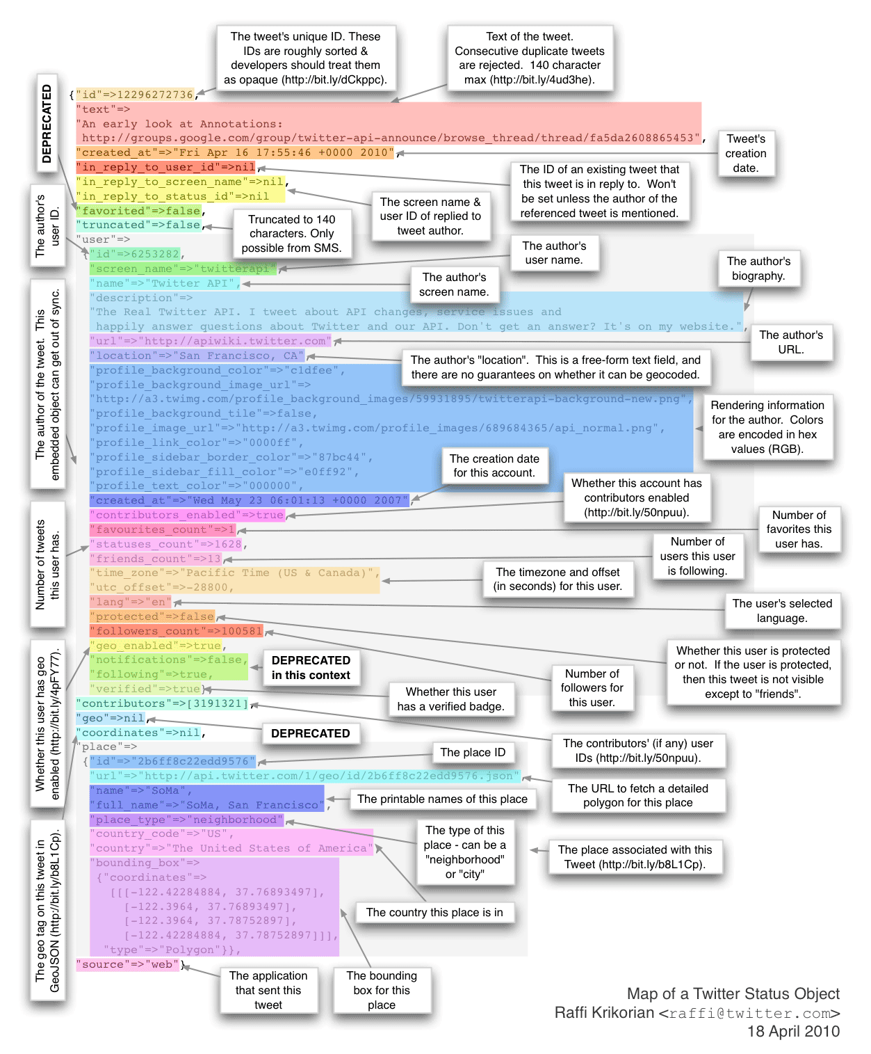
That might be a bit much, so just look at the top-level keys in the tweet object:
print tweet.keys()
You’ll see a list of keys: user, favorited, contributors, entities, text, created_at, truncated, retweeted, in_reply_to_status_id, coordinates, id, source, in_reply_to_status_id_str, in_reply_to_screen_name, id_str, place, retweet_count, geo, in_reply_to_user_id_str, and in_reply_to_user_id.
The id, text and time tweeted (“created_at”) are interesting. We’ll use “id_str” instead of “id” because Twitter’s numbers are so large that it’s generally more reliable to use string version than the numeric version. We can make a list of ID’s by looping over every tweet, like this:
ids = []
for tweet in tweets:
  ids.append(tweet['id_str'])
Since all we’re doing in this tutorial is looping over lists, it’s easier and faster to learn a feature of the Python language called list comprehensions. Carl Groner has an excellent explanation, as does Oliver Fromme. The short version is that these three lines are equivalent to three for-loops like the one above:
ids = [tweet['id_str'] for tweet in tweets]
texts = [tweet['text'] for tweet in tweets]
times = [tweet['created_at'] for tweet in tweets]
So now we have three lists: unique ID’s, text content (the actual words people wrote), and times for each tweet.
How about user information?
print tweet['user'].keys()
You’ll see another list of keys, with per-user information for each tweet: follow_request_sent, profile_use_background_image, geo_enabled, description, verified, profile_image_url_https, profile_sidebar_fill_color, id, profile_text_color, followers_count, profile_sidebar_border_color, id_str, default_profile_image, listed_count, utc_offset, statuses_count, profile_background_color, friends_count, location, profile_link_color, profile_image_url, notifications, profile_background_image_url_https, profile_background_image_url, name, lang, following, profile_background_tile, favourites_count, screen_name, url, created_at, contributors_enabled, time_zone, protected, default_profile, and is_translator. Twitter’s API saves you from having to look up extra information about each tweet by including it right there in every message. Although a tweet is only 140 characters, there can be as much as 4KB of data like this associated with each one.
We’ll just grab everyone’s name and screen name and leave the rest alone:
screen_names = [tweet['user']['screen_name'] for tweet in tweets]
names = [tweet['user']['name'] for tweet in tweets]
Looking for links, users, hashtags and places
When you tweet the “@” or “#” symbols or include links to web pages, these are interesting extra pieces of information. Twitter actually finds them for you and tells you exactly where in a message they are, so you don’t have to do it yourself. Look at the contents of a tweet’s entities object:
print tweet['entities']
You will see three lists: {'user_mentions': [], 'hashtags': [], 'urls': []}. For the tweet I chose, these are all empty. We’ll need to hunt through the full list of tweets to find one with a user mention, print it out and stop (“break”) when we’re done:
for tweet in tweets:
  if tweet['entities']['user_mentions']:
    print tweet['entities']['user_mentions']
    break
You may see something like this:
[
  {
    'id': 61826138,
    'id_str': '61826138',
    'indices': [0, 10],
    'screen_name': 'sabcab123',
    'name': 'Sabreena Cabrera'
  },
  {
    'id': 270743157,
    'id_str': '270743157',
    'indices': [11, 22],
    'screen_name': 'SimplyCela',
    'name': '(:'
  }
]
The two-element indices array says where that user mention begins and ends in the tweet; the rest of it is information about the mentioned user. In this case, I found a tweet with two users mentioned. Try doing the same thing for hashtags and urls. Links include Twitter’s shortened t.co link, the original fully-expanded address, and text that a client can display:
[
  {
    'indices': [39, 59],
    'url': 'http://t.co/XEvdU0cW',
    'expanded_url': 'http://instagr.am/p/PqMhTZtpw-/',
    'display_url': 'instagr.am/p/PqMhTZtpw-/'
  }
]
For every tweet in the list, we’ll pull out the first and second user mention, hashtag and link. Since many tweets may not have these and Python will complain if asked to retrieve and item in a list that doesn’t exist, we can use an if/else pattern in Python that checks a value before attempting to use it: thing if test else other_thing:
mentions1 = [(T['entities']['user_mentions'][0]['screen_name'] if len(T['entities']['user_mentions']) >= 1 else None) for T in tweets]
mentions2 = [(T['entities']['user_mentions'][1]['screen_name'] if len(T['entities']['user_mentions']) >= 2 else None) for T in tweets]
hashtags1 = [(T['entities']['hashtags'][0]['text'] if len(T['entities']['hashtags']) >= 1 else None) for T in tweets]
hashtags2 = [(T['entities']['hashtags'][1]['text'] if len(T['entities']['hashtags']) >= 2 else None) for T in tweets]
urls1 = [(T['entities']['urls'][0]['expanded_url'] if len(T['entities']['urls']) >= 1 else None) for T in tweets]
urls2 = [(T['entities']['urls'][1]['expanded_url'] if len(T['entities']['urls']) >= 2 else None) for T in tweets]
At the beginning of this exercise, we used a geographic bounding box to search for tweets—can we get the geographic location of each one back? We’ll start with just a point location:
print tweet['geo']
Which gives us something like {'type': 'Point', 'coordinates': [40.852, -73.897]}. So, we’ll pull all the latitudes and longitudes out of our tweets into two separate lists:
lats = [(T['geo']['coordinates'][0] if T['geo'] else None) for T in tweets]
lons = [(T['geo']['coordinates'][1] if T['geo'] else None) for T in tweets]
Twitter also says a little about the place where a tweet was sent, in the place object:
print tweet['place'].keys()
The keys on each place include country_code, url, country, place_type, bounding_box, full_name, attributes, id, and name. We’ve already got geographic points above, so we’ll just make a note of the place name and type:
place_names = [(T['place']['full_name'] if T['place'] else None) for T in tweets]
place_types = [(T['place']['place_type'] if T['place'] else None) for T in tweets]
Outputting to CSV
We’ve collected fifteen separate lists of tiny pieces of information about each tweet: ids, texts, times, screen_names, names, mentions1, mentions2, hashtags1, hashtags2, urls1, urls2, lats, lons, place_names and place_types. They’re a mix of numbers and strings and we want to output them someplace useful, perhaps a CSV file full of data that we can open as a spreadsheet or insert into a database.
Python makes it easy to write files. Start by opening one and printing a line of column headers:
out = open('/tmp/tweets.csv', 'w')
print >> out, 'id,created,text,screen name,name,mention 1,mention 2,hashtag 1,hashtag 2,url 1,url 2,lat,lon,place name,place type'
Next, we’ll let the built-in csv.writer class do the work of formatting each tweet into a valid line of data. First, we’ll merge each of our fifteen lists into a single list using the indispensable zip function. Then, we’ll iterate over each one taking care to encode our text, which may contain foreign characters, to UTF-8 along the way:
rows = zip(ids, times, texts, screen_names, names, mentions1, mentions2, hashtags1, hashtags2, urls1, urls2, lats, lons, place_names, place_types)

from csv import writer
csv = writer(out)

for row in rows:
    values = [(value.encode('utf8') if hasattr(value, 'encode') else value) for value in row]
    csv.writerow(values)

out.close()
Boom! All done. You now have a simple file that Numbers, Excel and MySQL can all read full of sample tweets pulled directly from the live, streaming API.
Sep 9, 2012 2:25am
generating repeating patterns
I’ve been looking at the Gray-Scott Model of reaction-diffusion, and thinking about how to use it to create natural-looking, repeating patterns.

From Rob Munafo’s page on R-D:
All of the images and animations were created by a computer calculation using the formula (two equations) shown below. …the essence of it is that it simulates the interaction of two chemicals that diffuse, react, and are replenished at specific rates given by some numerical quantities. By varying these numerical quantities we obtain many different patterns and types of behavior.
My quick pattern explorations were the result of some unsharp mask tweaking, but they’re all results of the output of a simple python script using a range of input F and k parameter values. The raw outputs look a little like this:

The variation in output is pretty astonishing, from the worms-and-blobs above to a tanned-leather dimple, earthworm maze, or Mayan-looking interlock:


Over about a week of computer time, I’ve generated 300+ renderings of a particular interesting portion of Munafo’s high level view as 1024x1024 tileable patterns:

Jun 26, 2012 6:39am
cascadenik in 2012
I went on a tear with Cascadenik in May and June, here are three cool new things you can do with it.
1. Use Mapnik 2
Artem, Dane and company have been diligently pushing Mapnik forward, and this spring saw the inclusion of Mapnik 2 in the newest Long Term Support version of the Ubuntu operating system, Precise Pangolin. Mapnik 2 has a variety of under-the-hood optimizations in stability and speed and an improved approach toward backward and forward compatibility, so it’s exciting to get Cascadenik back in synch with its host program.
2. Make Retina Tiles
Apple’s moving toward high resolution Retina display on all its hardware, and the usual doubling of old-resolution graphics can look pretty terrible. Cascadenik now has a built-in “scale” parameter, exposed as the “2x” flag to the compile script. You can painlessly double the resolution of an output and adjust all the scale rules, generating Retina-ready stylesheets at twice the visual resolution.
Retina version:

(both examples from OSM-Solar)
3. Write Concise Stylesheets
Carto picked up a few interesting features from Less-CSS, and Cascadenik now has versions of two of them.
Nested rules can simplify the creation of complex styles, making it easier to build up combinations of selectors over many sub-styles or zoom levels. Check out a particularly pathological example from Toner that shows how to separate general text attributes from zoom-specific ones. Cascadenik’s interpretation of Less is a bit stricter than Carto’s, which mostly just means that you have to add a few ampersands.
Variables are a simple way to group things like color or font selections in a single part of a stylesheet. While this isn’t something I use much of, it was an oft-requested feature and may make its way into Toner to enable simple customization. They work pretty much as you’d expect, taking on the precedence of where they’re used rather than where they’re defined.
I’m working with Nathaniel Kelso to identify other must-haves from Mapnik to include in Cascadenik, and as always focusing on stability and interoperability with other parts of the map building stack from data preparation tools like Dymo and Skeletron to eventual rendering and serving via TileStache.
Apr 25, 2012 10:25pm
polygonize it
If you need to make a bag of polygons from a selection of OpenStreetMap data, you would think that simply running shapely.ops.polygonize on the selection of linestrings is enough. In fact, polygonize needs for the line endings to coincide, and may not work as you would expect with OSM data. I scratched my head over this a bit after successfully using polygonize to handle TIGER data, until it occurred to me that TIGER is built to have lots and lot of little lines.
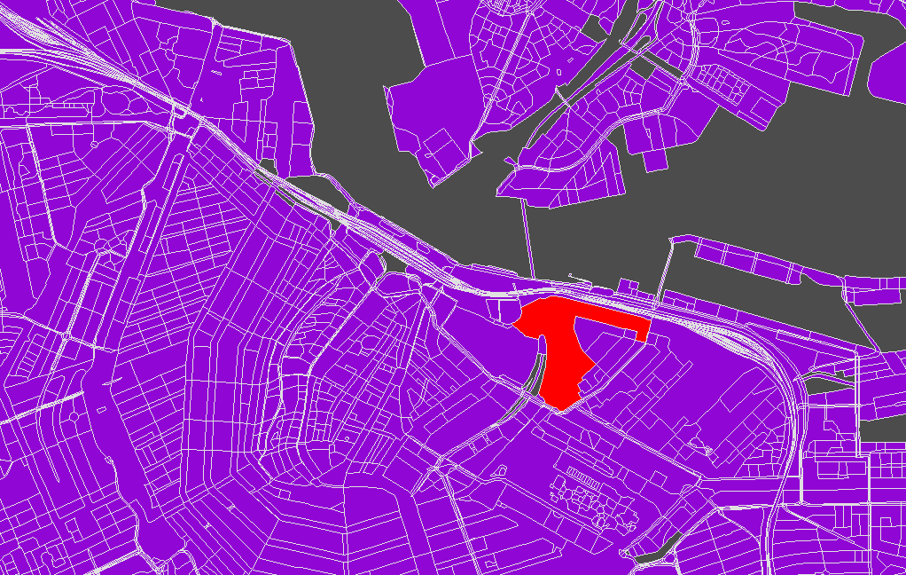
The trick is to split each linestring input to polygonize() into all its constituent segments, and then let the function do the reassembly work for you. Creating the polygons of Amsterdam above from metropolitan extract roads took just a few seconds. Here’s the polygonize.py script that does it, expecting GeoJSON input and producing GeoJSON output.
Apr 16, 2012 5:54am
hachures
Hachures are an old way of representing relief on a map. They usually look a bit like this, and they’re usually hand-drawn:
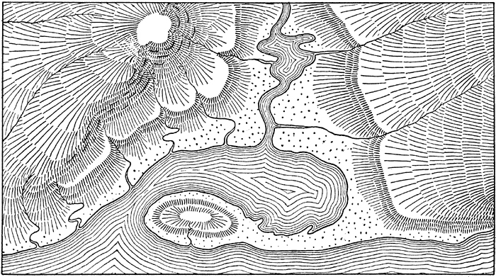
I’ve been playing some some simple algorithmic ways to generate hachure patterns with input elevation data.
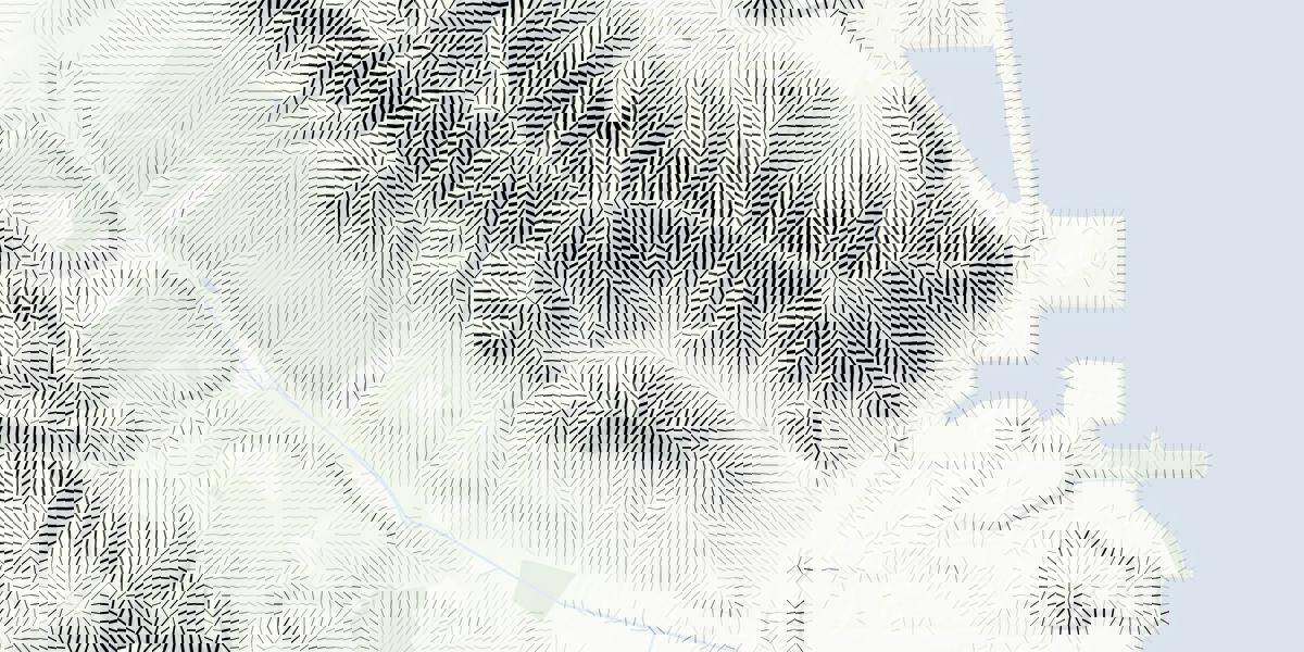

They’re rather New Aesthetic, with the regular-spaced grid based this pattern that encodes slope and aspect together:

You can align the marks with the slope, or across it (as with contour lines). The latter results in some pretty blocky-looking hills; my feelings about these are mixed:

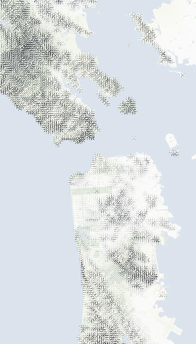
I especially enjoy the smooth appearance of hills in San Francisco using the orientation along the slope. Things get even more interesting when minimal labels are added on top:

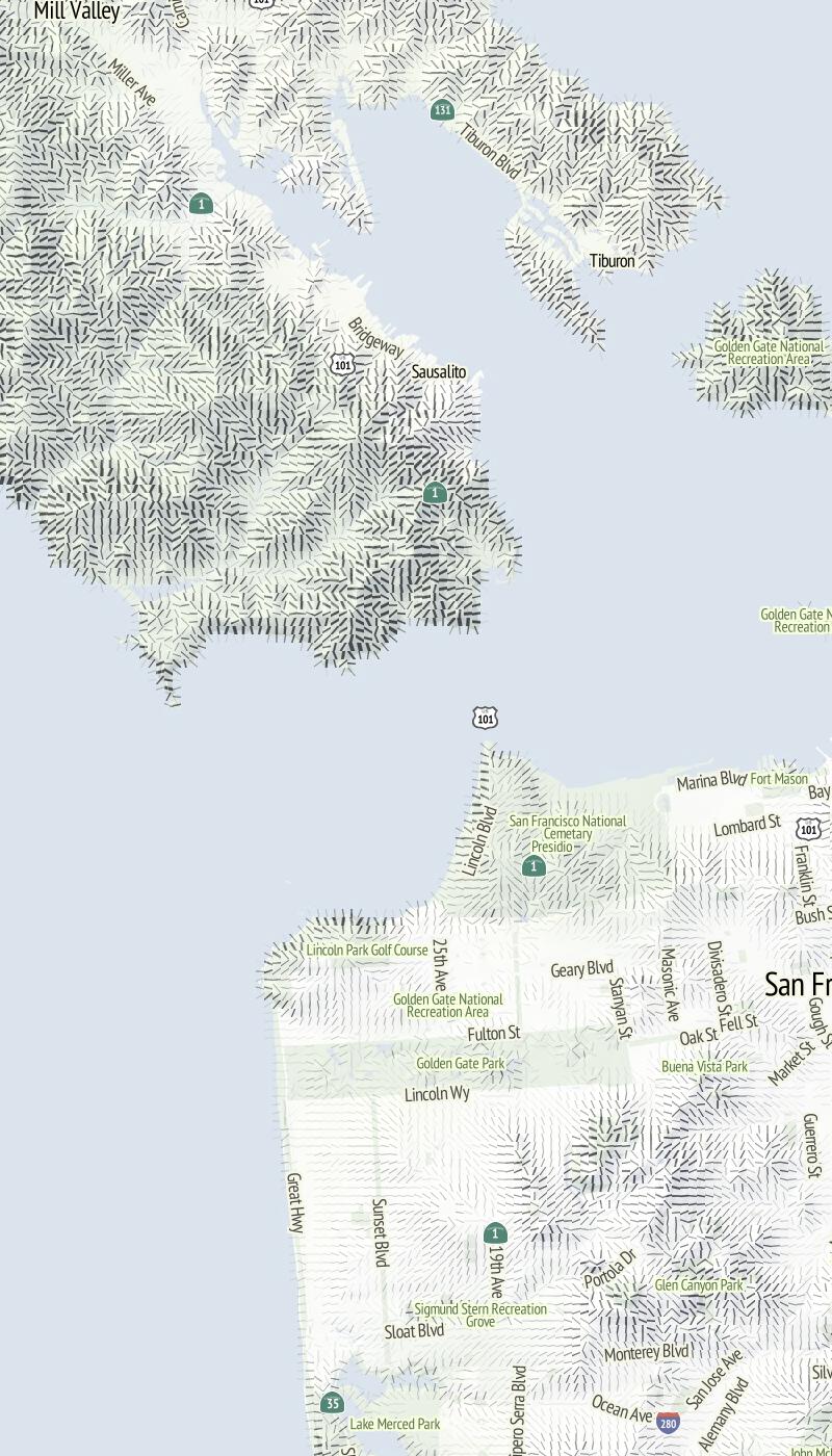
Also, good things happen at relative-low zoom levels, where the relative size of hills and marks gives everything a spiny, written-on appearance:
Have a look through a collection of renders for more examples.
Apr 9, 2012 6:02am
chicago-bound
Next weekend, I’m heading to Chicago to spend a week volunteering for the Obama 2012 campaign’s tech team. I’m very excited; it should be a fairly high pressure environment and I hope to have a number of opportunities to bring a bit of API design and basemap cartography love from San Francisco.
This election feels intuitively like the one that matters, the one where we prove that the past four years weren’t just a reactionary fluke. We had a round of flowers and sunshine last time around, but the President wasn’t running on much of a record. In 2012, he’s been in office for a full term, and a lot of people who were hoping to see a 180° turnaround from the Bush years were disappointed to discover that ours is a rough political landscape to navigate. Given the circumstances, I think Obama’s done a great job. Given the risk that supporters from 2008 might not be so excited this time around, I’m putting in extra energy to help assure that we can push this not-at-all-guaranteed election over the hump.
If you’re local to San Francisco and want to help, Catherine and Angus at the SF technology field office in SOMA are looking for your help.
Apr 4, 2012 6:11am
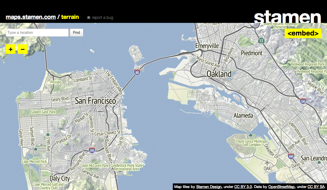
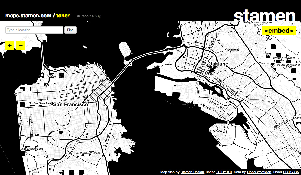
maps.stamen.com
We launched a thing last week. It was fairly well-received by people on the internet. A few people at Stamen who don’t normally write on the company blog wrote on the company blog: Zach talked about the blur/noise process behind the watercolor tiles, Geraldine explained all the work that went into the textures, and Jeff showed off some of his work logging tile usage on the site. I recapped a lot of my background work on Terrain, and then Cups And Cakes Bakery went and made it into cupcakes.
Paul Smith, who taught me how to install Mapnik a long time ago, did an interview with me about maps while slacking off from his day job. In it, I wrote a bunch of things that I think are interesting about online maps, which is a good thing because today I didn’t feel well and bailed on my Where 2.0 talk. Sorry about that—you didn’t miss anything, I was really unhappy with the talk I had prepared, which probably contributed to my morning.
Here are pictures:

Mar 19, 2012 8:00am
tinkering with webgl
With some help from Ryan and Tom, I’ve been wrapping my pea-sized brain around WebGL. I’m doing my usual start-from-the-bottom thing so it’s been a great exercise in understanding a programming paradigm built around static lists and buffers. I’ve worked like this before, but not extensively and not with a render output this smoking fast.
It’s all simple stuff so far, but I’m chasing two ideas: using WebGL for simple 2D output with an added speed bump, and driving it from SVG or the HTML DOM. None of the examples below will work unless you’re using a current WebGL-compliant browser, which for me was Chrome 17.
The elephant is me figuring out the basics of viewport transformations that match pixel positions, image textures, and simple animation passed via vertex buffers:

The monkey is a test to see how many things I can throw around on a screen without sacrificing framerate, as well as some sanity checks on coding style. Turns out, the answer is “lots”. Interesting things happen with this one when you switch to and from its tab; I’m using a basic timeout-based mechanism for the little face particles, and it clearly falls into a regular rhythm.

The unicode patterns (borrowed from Sarah Nahm) are governed by an invisible D3 force layout, and are a test of synchronization between multiple “programs” and driving a visual effect from a geometric layout. Also additive blending for punchiness. Try dragging the boxes:

These are some of the resources I’ve been using to get up to speed:
- Learning WebGL
- OpenGL Shading Language wiki
- CAAT implementation notes
- Mozilla Developer Network (with best practices)
- Raw WebGL from Opera
I’m still not totally comfortable with the programming approach of maintaining collections of static lists in preference to objects and other data structures, and I’ve been avoiding three.js until I can get comfortable with how WebGL works for simple, two-dimensional graphics. No lighting effects or spinny statues quite yet.
Mar 11, 2012 6:39pm
county papers
I’ve been playing with ways to represent U.S. OSM involvement at the county level. This is in part spurred by some of Thea Aldrich’s work since the last State Of The Map U.S. as well as by Martijn Van Exel’s Temperature of local OpenStreetMap Communities. The county-equivalent is a basic unit of administrative power, a common baseline for Census demographic statistics, often home to GIS professionals, and guaranteed to cover any given piece of land in the United States. It’s a great way to divide a dataset like OpenStreetMap, so I’ve started to experiment with useful print representations of counties for looking at map coverage.

(PDF download, 21MB)
The visual design is rather primitive so far, with just three maps on a single tabloid printout as a quick test. At top is a basic representation of OSM coverage, a sort of “what do we know” for streets. Next is a map of TIGER/Line status, highlighting streets which remain untouched since their initial import in 2007 and probably overdue for review. Finally, a map showing recently-edited streets, which looks a little more interesting the Austin, Texas render. Each is rendered using Mapnik and Cairo’s PDF output from a recent OSM Planet extract.
There are intentional echoes of Newspaper Club’s Data.gov.uk Newspaper here.
My afternoon test prints suggest a few things:
- Printers have a very hard time with fine linework, so I’m switching to halftones for the smaller maps.
- I need to get many more layers of information in there, including buildings, parks, points of interest, etc.
- Maps will look better when printed large.
- I should do a newspaper run like Grassroots Mapping did recently, the output looks great:

Code can be found in Github under CountyOSM. You are not expected to understand it.
Mar 9, 2012 5:16pm
“nice problem to have”
A mail from OSM Board member Richard Fairhurst, to the OSM-Talk mailing list about Apple’s recent use of our data, with links added for posterity:
3500 tiles per second. Seriously. In Grant’s words on Twitter: “Massive jump in #OpenStreetMap traffic due 2 Apple news: t.co/nB4ffgYy Fighting fires 2 keep systems up”
switch2osm.org fell over. Yep, so many people wanting to find out about switching to OpenStreetMap that WordPress crapped itself (ok, not the hardest target but hey ;) ).
More contributors. We’ve had people come into IRC saying “I want to fix this park name, how do I do it?”. Regular IRCers have been reporting a noticeably greater number of new editors in their areas. Or as someone just asked on IRC: “hmm did the apple fanbois drink the OSM koolaid and crash our servers with zealous mapping?”
I think we’ve had a higher peak of publicity today than we’ve ever had —higher than the Foursquare switch even, or the Google vandalism incident. We’ve been Slashdotted; we’re #6 on Hacker News. We’ve been on The Verge, Forbes, Wired, Ars, Gizmodo, and all the Mac sites—that’s taking OSM to people who’ve not heard of us before. We might not be the front page of the New York Times yet, but we’re getting there!
And one of the best things has been that people like how we’ve handled it. From Forbes: “OpenStreetMap itself has been much more polite about the whole thing. ‘It’s really positive for us,’ OSM founder Steve Coast told Talking Points Memo, ‘It’s great to see more people in the industry using OSM. We do have concerns that there wasn’t attribution.’.”
From a comment at Hacker News: “While I think it’s quite messed up that a company as rich as Apple can’t abide putting credits for people who have put some really good work in (I’ve even made small updates to OSM in my time) I do think that this is a very classy move by the OSM people, no ranting blog post or ‘Apple stole our stuff’, welcoming people presents a much better image of the project.”
Or The Verge: “Granted, OSM took this as an opportunity to get in the public eye by piggybacking on the iPad’s media fanfare; I applaud them for their maturity in their statement though. Many companies would’ve latched onto this and unleashed the lawyers threatening this and that, but they chose to be civil, point out the missing attributions, and say they are ‘we look forward to working with Apple to get that on there.’ A little civility goes a long way (in my book). I’m quite sick of the mudslinging in this space.”
Thanks to everyone who’s put the hours in today, to all the coders and sysadmins who sweat blood to not only keep OSM running but make it easier and faster... and to every single mapper making a map so amazing that everyone wants to use it.
cheers
Richard
Mar 6, 2012 7:49am
2sleep1
I am kinda losing my mind over this hour-plus ambient audio/video construction by Goto80 and Raquel Meyers:
Press play, go fullscreen and lie down. 2SLEEP1 is a 66-minute playlist of audiovisual performances in text mode, designed to make you fall asleep. Made by Raquel Meyers and Goto80.
The first and fourth tracks are especially genius.


Mar 4, 2012 1:41am
bandwidth
Webkit size profiles of a few sites I visit, ordered from smallest to largest.
Metafilter: 0.2MB

Metafilter’s front page is probably my most-visited and most-interesting thing. It’s a wall of solid text and not a lot of images. Still, the volume of actual content is smaller than the volume of javascript, which itself is about 80% jQuery (minified). It’s not immediately clear to me what jQuery is doing for Metafilter.
Google Homepage: 0.5MB

I don’t actually visit Google.com much and I typically have Javascript suppressed for the domain when I do, but the default experience looks like this: half a megabyte, 60% of which is a single .js file clocking in at 300KB.
OpenStreetMap: 0.64MB

The bulk of OSM’s Javascript use is taken up by OpenLayers, an epic bandwidth hog coming in at 437KB minified. You can build custom, minified versions of OpenLayers with just the features you want; I’ve never successfully gotten one below 250KB. Based on my experience with Modest Maps, I think it should be possible to get the core functionality of OpenLayers across in 100KB, tops. The next 100KB of Javascript on this site is a minified archive of Sizzle and jQuery. The remaining 16% of the bandwidth for this page is the visible map and all other content.
New York Times: 0.76MB

The Times is a toss-up depending on when you’re looking at it; I just reloaded and saw the overall size jump to 1.4MB, then reloaded again and saw it drop to 0.5MB. It’s the front page of a major paper, so the ratio of actual content (text and images) to code and stylesheets looks to be in the 2 or 3 to one range, which is decent.
Github, My User Page: 0.99MB

I spend an inordinate amount of time on Github these days. It’s balanced heavily toward code and stylesheets, with about a three-to-one ratio of framework to content. Github’s Kyle Neath has an excellent presentation on responsive web design where he shows how despite the heavy load of Javascript and CSS used in Github’s interface, the all-important “time to usable” metric is still pretty fast for them. He contrasts this to Twitter, which… ugh, more on them below.
My Home Page: 1.1MB

Here’s me; essentially 100% Actual Content, mostly images. I switched to big, stretchy images a little while back, and I’ve gotten more free with the sizes of things I post.
The Awl: 1.36MB

Page sizes take a sharp upward tick here. Most of The Awl is Javascript, though it appears to be largely custom with the usual slug of jQuery sitting in the middle. A majority comes from widgetserver.com and ytimg.com, so I’m going to guess it’s lightboxes and ad server junk.
The Verge: 7.4MB

Lots and lots of pictures. So many that after a minute or two, I wondered whether something had gone wrong with my network connectivity. Below all the images, there is 300KB of minified jQuery, thanks to the inclusion of jQuery UI. Also, 244KB of fonts which in Safari prevents any text from loading until this item is done.
A Single Tweet: 2.0MB

Twitter allows you send 140 characters in a tweet, which (when you add entities, hashtags, and all that) ends up in the 4KB range as represented in the JSON API. 140 is what you see, so I’m going to go out on a limb and suggest that a single tweet page on Twitter has about a 15,000-to-one ratio of garbage to content.
I get links to tweets by mail, etc. on a regular basis, and the aggressive anti-performance and apparent contempt for the web by Twitter’s designers is probably the thing that gets me most irrationally riled-up on a daily basis. How does this pass design review? Who looks at a page this massive, this typically broken and says “go with it”?
It’s mind-boggling to me that with the high overlap between web developers/designers and iPhone users on AT&T’s network, there isn’t more and smarter attention paid to the sizes of the things we’re slinging around the network. The worst sins of the Flash years are coming back with a vengeance, in the form of CSS Frameworks and the magic dollar sign. There has seriously got to be a better way to do this.
Feb 26, 2012 10:57pm
tile drawer: grist for the mill
Last week, I finished up my four-part class at GAFFTA on visualizing and mapping data. For day three, I chose Mapbox’s TileMill to teach basic cartographic techniques such as choropleths and managing data from OpenStreetMap. I’d never really used TileMill in anger, and teaching the class was an excellent opportunity to apply experience with Mapnik and Cascadenik to a tool built for normal humans to use. I can report that TileMill is a champ. It’s not often that advanced nerd tools are adapted for civilian use, and the group at Development Seed have done an amazing job of packaging the Mapnik experience into a credible desktop application for easy cartography.
Meanwhile, Tile Drawer is now over two years old, and the stars are aligning for a revisit. I’ve substantially updated and modified Tile Drawer for the end times, and I’ve been retooling the creation process to address two questions that TileMill raises: how do you get data from OpenStreetMap in to begin with, and then what do you do with your tiles when you’re done? MapBox answers the second question with their various hosting plans, but what if you want to serve maps for areas larger than a single MBTiles files can handle or you simply want to be ready for the kinds of futures envisioned by Maciej Cegłowski or Aaron Cope?
I’ve been slowly and quietly answering the first question by building up shapefile exports for my Metropolitan Extracts service, and I’m happy to announce that it now includes Imposm and Osm2pgsql shapefiles for every extracted area. Oliver Tonnhofer’s Imposm is particularly well-suited to use in Tilemill, with its thematic division of OSM data into thematic layers.
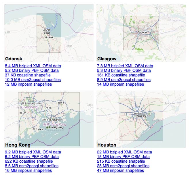
If you want to use OSM data in Tilemill, and you’re interested in one of the 130+ extended metropolitan areas I’ve been supporting in the Metro Extracts, then you should be good to go with the zip files available there.
Now, about that second question.
I’ve generated collections of data in specially-named shapefiles for four sample metro areas:
- San Francisco (just osm2pgsql, just imposm)
- London (just osm2pgsql, just imposm)
- Berlin (just osm2pgsql, just imposm)
- Tokyo (just osm2pgsql, just imposm)
If you use these files with their names unchanged in TileMill and supply a zip file of your exported Mapnik 2.0 XML stylesheet to Tile Drawer, it will be able to figure out what PostGIS tables you might mean and render a map accordingly. If you want a map layer for all of Texas, it would probably take too long to render the entire set of tiles using TileMill and too long to upload it all to MapBox. Instead, you can start with a sample city above, create a custom cartographic treatment in TileMill, and then provide Tile Drawer with a bounding box for the entire state and a copy of your stylesheet. I’ll be documenting this process on the site soon for more information.
Looping back around, Tile Drawer is useful for TileMill even if you plan to use Mapbox for hosting. One of the last things that Tile Drawer does after importing a data extract is to generate the same collection of Osm2pgsql and Imposm shapefiles available in the sample selections above, so you can prepare data for your own use by setting up an instance of Tile Drawer, waiting for it to finish importing data from OpenStreetMap, and then downloading one of the osm-shapefiles zip files found in /usr/local/tiledrawer/progress.
Jan 9, 2012 5:27am
take my class at gaffta next month
I’ll be teaching a four-day class at the Gray Area Foundation For The Arts next month, Visualizing and Mapping Data. It’ll be a four-parter, Tuesday and Thursday evenings at GAFFTA’s San Francisco space. I’ll be covering mapping from both a browser and server perspective, focusing the presentation of data.

Here’s an early draft of my class notes; these will change but not substantially:
This four-day workshop will follow the lifecycle of data, from its raw collection to preparation and presentation for the web. We’ll explore where geographic data originates, how it’s transformed to work online, how to see it flow and move, and finally how to publish a view into that data to the web with simple browser-based tools. We’ll work with data from Twitter and OpenStreetMap, push it through filters and viewers, and publish it to the open web.
This class will cover both browser-side Javascript code and server-side Python code.
Week One: Foregrounds
Meeting 1: Getting dots on maps
We’ll be working with street-level data for the duration of the class, so we’ll start here with some introductory concepts like interactive slippy maps and image tiles. We’ll take Google Maps apart into its component pieces to see how they work, add a selection of point-based data to a map, and finish up with a working example using freely-available Javascript mapping tools.
Meeting 2: Where data comes from
Data can come from all kinds of sources, and frequently it needs to be processed, cleaned, and prepared for use on the web. Become self-sufficient in making location data useful to others. We’ll look at local data sources like 311 calls, addresses, and demographic information and run them through a variety of tools to make them ready for online publishing.
Week Two: Backgrounds
Meeting 3: Choosing your own background
Commonly-available road maps designed for displaying driving directions or finding business addresses don’t always work in combination with arbitrary or complex data. We’ll look at alternate sources of street-level cartography and talk about the ways each might be appropriate to different data sets. We’ll finish up with a dive into the OpenStreetMap data set and the process of designing your own custom cartography.
Meeting 4: Spatial data
Dots on maps are just one of many ways to display data. Heat maps, for example, can be used to show characteristics of large areas of data such as zip codes or census tracts using color. We’ll look at ways to prepare heat map layers and integrate them with our other maps, and finish up with advanced topics like aerial photographs and raster data.
Jan 8, 2012 9:08am
new webgl nokia maps: progress
I’ve been kicking some files from the new Nokia 3D WebGL maps back and forth with Ryan Alexander, and my attempts to pick out the geometry are starting to get some results.
Nokia’s texture files:

My points in those same files—a visual match!

Dumping a bunch of X, Y, Z’s into Mac OS X Grapher.app:
Ryan pushing the whole thing into Blender:
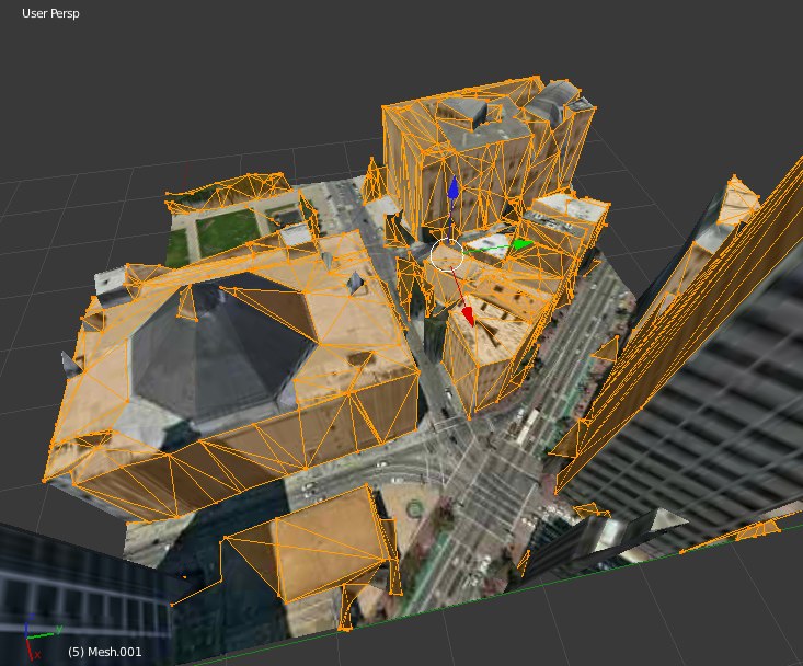
This model is actually two meshes, corresponding to two separate textures:


The first one looks a bit like a post-Tornado city. Now to figure out the mipmaps in the height lookup tables.
Jan 6, 2012 12:25am
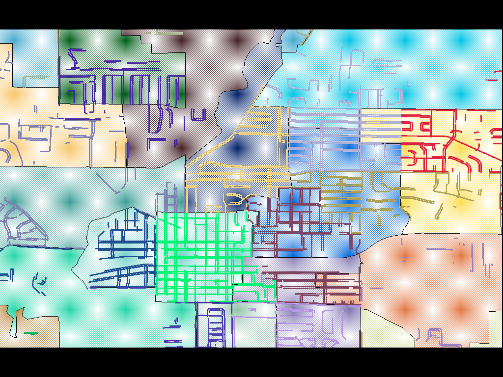
new webgl nokia maps
Nokia’s new 3D WebGL maps are done very nicely. Here’s my house:

Here’s the zoom=16 texture JPEG for the are around my house:
And here are parts of the raw geometry for the same area. I'm thinking to do as Brandon Jones did and figure out the file format here, since I can already see obvious signs of four-byte floating point values:
00000000  4e334d34 01000000 01000000 28000000  N3M4........(...
00000010  97160000 f4c30100 82120000 00000000  ................
00000020  84330200 a0330200 00d01345 0040f644  .3...3.....E.@.D
00000030  003f3947 00001745 00c02845 00572f47  .?9G...E..(E.W/G
00000040  00a03045 0068e245 006e3947 9e080545  ..0E.h.E.n9G...E
00000050  1a920346 66f33447 00501745 00003442  ...Ff.4G.P.E..4B
00000060  00a93247 00901645 00003442 00b83447  ..2G...E..4B..4G
00000070  00602145 00003442 00164147 00e00a45  .`!E..4B..AG...E
00000080  00c8e845 00272947 00801645 0070f545  ...E.')G...E.p.E
00000090  00994347 00a01245 00982846 004d3547  ..CG...E..(F.M5G
000000a0  00102245 00e43346 00874447 00300c45  .."E..3F..DG.0.E
000000b0  00587346 00fd3047 00c0fc44 00cc7746  .XsF..0G...D..wF

...

00010f20  68cb1f47 07d54c44 89405f47 d4853f47  h..G..LD.@_G..?G
00010f30  42035044 5c405f47 31405f47 b9e8383e  B.PD\@_G1@_G..8>
00010f40  aff0ae3e d4b0533e b0caaf3e c40c443e  ...>..S>...>..D>
00010f50  c944c93e 3003523e 9ee0cd3e c568453e  .D.>0.R>...>.hE>
00010f60  a37ea33e c02c403e a412a43e a1c4203e  .~.>.,@>...>.. >
00010f70  a88aa73e eed86d3e c6bac53e ac8c2b3e  ...>..m>...>..+>
00010f80  cf28cf3e d658563e dac6d93e b140313e  .(.>.XV>...>.@1>
00010f90  e2a4e13e ecd06b3e f068f03e f940793e  ...>..k>.h.>.@y>
00010fa0  f06af03e 8188803e d5b4d43e 898c883e  .j.>...>...>...>
00010fb0  863f063f 8588843e ca84c93e 9040903e  .?.?...>...>.@.>
00010fc0  c7c8c63e a0f09f3e c3bec23e 8a748a3e  ...>...>...>.t.>
00010fd0  c49ec33e 91a2903e bf40bf3e 9028903e  ...>...>.@.>.(.>

...

0001c3c0  8b0b503f c40d053f e87d543f eacce13e  ..P?...?.}T?...>
0001c3d0  91f1583f 034da53e 459e5f3f 917fb93e  ..X?.M.>E._?...>
0001c3e0  98635d3f 6732913e 36d6613f 1fca513e  .c]?g2.>6.a?..Q>
0001c3f0  1e49663f b913ba13 c900b913 c9006213  .If?..........b.
0001c400  b9136213 6113bb13 bd13cb00 bb13cb00  ..b.a...........
0001c410  ca00bd13 be13cb00 be13bf13 cb00bf13  ................
0001c420  cf00ce00 d000ce00 cf00d300 ce00d000  ................
0001c430  d300d400 ce00d400 d300d500 d400d500  ................
0001c440  d600d700 d400d600 d600d800 d700d400  ................
0001c450  d700d900 d900da00 d400db00 da00d900  ................
0001c460  d800d600 dc003802 39023a02 39023802  ......8.9.:.9.8.
0001c470  3b023902 3b023c02 76137713 39027613  ;.9.;.<.v.w.9.v.
0001c480  39023c02 1f032003 21031f03 22032003  9.<... .!...". .
0001c490  23032203 1f032303 24032203 79137a13  #."...#.$.".y.z.
0001c4a0  1a047a13 1d041a04 7a137b13 1e047a13  ..z.....z.{...z.
0001c4b0  1e041d04 71067206 73067406 73067206  ....q.r.s.t.s.r.
0001c4c0  75067306 74061407 15071607 16071707  u.s.t...........
0001c4d0  14071807 16071507 16071807 19071907  ................
0001c4e0  18071a07 d008d108 d208ea13 eb13d508  ................
0001c4f0  ea13d508 d308d608 d308d508 3b093c09  ............;.<.
0001c500  3d093c09 3e093d09 a10aa20a a30aa10a  =.<.>.=.........
0001c510  a40aa20a a20aa40a a50ac30a c40ac50a  ................
0001c520  c50ac60a c30ac50a c40ac70a c40ac80a  ................
0001c530  c70a9513 9613230b 9513230b 210be00c  ......#...#.!...
0001c540  e10ce20c a213a413 ec0ca213 ec0cea0c  ................
0001c550  0a140b14 010d0a14 010dff0c 2c0e2d0e  ............,.-.
0001c560  2e0eb90e d000cf00 b90eba0e d000bf0e  ................
0001c570  d300d000 bf0ec00e d300c10e d500d300  ................
0001c580  c10ec20e d500c30e d600d500 c30ec40e  ................
0001c590  d600c50e d700d800 c50ec60e d700c70e  ................
0001c5a0  d900d700 c70ec80e d900c90e db00d900  ................
0001c5b0  c90eca0e db00cb0e dc00d600 cb0ecc0e  ................
0001c5c0  dc00cd0e d800dc00 cd0ece0e d800210f  ..............!.
0001c5d0  3b023802 210f220f 3b02230f 3c023b02  ;.8.!.".;.#.<.;.
0001c5e0  230f240f 3c027813 3c02250f aa137813  #.$.<.x.<.%...x.
0001c5f0  250fc110 2c0e2e0e c110c210 2c0e2014  %...,.......,. .
0001c600  b9136113 78137613 3c027b13 7c131e04  ..a.x.v.<.{.|...
0001c610  80137f13 55068013 55065606 7f138113  ....U...U.V.....
0001c620  55068313 82137607 82138413 77078213  U.....v.....w...
0001c630  77077607 8f138e13 1d098f13 1d091e09  w.v.............
0001c640  9c139b13 660c9c13 660c670c 9b139d13  ....f...f.g.....
0001c650  660ca313 a213ea0c a313ea0c eb0cbc13  f...............
0001c660  bb13ca00 bf13ce00 cb00bf13 c013cf00  ................
0001c670  c0131014 bc0ec013 bc0ecf00 c100c400  ................
0001c680  0800c600 0800c400 c400c700 c6007613  ..............v.
0001c690  78133e02 76133e02 3d023d02 3e023f02  x.>.v.>.=.=.>.?.
0001c6a0  3f024002 3d023f02 41024002 41024202  ?.@.=.?.A.@.A.B.
0001c6b0  40024102 3f024302 43024402 41024102  @.A.?.C.C.D.A.A.
0001c6c0  44024502 44024302 46024702 44024602  D.E.D.C.F.G.D.F.
0001c6d0  41024802 42025703 58035903 58035703  A.H.B.W.X.Y.X.W.
0001c6e0  5a035b03 57035903 5c035803 5a035c03  Z.[.W.Y.\.X.Z.\.
0001c6f0  5d035803 5a035d03 5c031c13 1b13ae03  ].X.Z.].\.......
0001c700  7c137b13 1c047c13 1c041f04 6e056f05  |.{...|.....n.o.
0001c710  70057005 71056e05 71057005 72057f13  p.p.q.n.q.p.r...
0001c720  80135406 81137f13 54068113 54065706  ..T.....T...T.W.
0001c730  27132813 1d072713 1d071b07 1d071e07  '.(...'.........

...

00023250  08118916 08119d00 86115400 05118611  ..........T.....
00023260  05110611 07110511 5400e211 86110611  ........T.......
00023270  e511e211 0611e511 06117d11 90168b16  ..........}.....
00023280  54009016 54008511 86118511 54008a16  T...T.......T...
00023290  8f160711 8a160711 54008b16 8a165400  ........T.....T.
000232a0  05119c00 9b008916 88169c00 89169c00  ................
000232b0  05118916 05110711 8f168916 07110611  ................
000232c0  9b00af0e 7d110611 af0eb10e 9b009c00  ....}...........
000232d0  b10eb20e 9b00b50e 9c009f00 b50eb60e  ................
000232e0  9c000611 05119b00 88169f00 9c008816  ................
000232f0  8d169f00 8d168e16 b40e8d16 b40e9f00  ................
00023300  03000000 6c000a01 7201b301 0b028f02  ....l...r.......
00023310  ca021f03 8d03d003 5504c904 04055505  ........U.....U.
00023320  9005c205 3906a506 f8067907 da076608  ....9.....y...f.
00023330  98080709 6209c609 fe09510a b00a310b  ....b.....Q...1.
00023340  8f0b4d0c b20c150d 5d0d8d0d cd0df80d  ..M.....].......
00023350  220e460e 680e790e 850eae0e b60ebe0e  ".F.h.y.........
00023360  e60e200f 470f940f af0fc80f 5e10f310  .. .G.......^...
00023370  5011d211 da11e011 f7110d12 28126612  P...........(.f.
00023380  72120000 186d6170 5f31365f 34303231  r....map_16_4021
00023390  325f3130 3531305f 302e6a70 67000000  2_10510_0.jpg...
000233a0  40bf5aba 8940adba 78f89e3a 00000000  @.Z..@..x..:....
000233b0  5a48ce3b c23982bb 00000000 00000000  ZH.;.9..........
000233c0  a8fb1e3b e6d57b3b c3ebbf3b 00000000  ...;..{;...;....
000233d0  456924ca f93382ca 4a546d4a 0000803f  Ei$..3..JTmJ...?
000233e0  00ffff46 00ffff46 00ffff46 00ffff46  ...F...F...F...F
000233f0  00ffff46 00ffff46 5f1d1508 e8574bbf  ...F...F_....WK.
00023400  b648222b 11a855bf 7a5ef80a 0fdf533f  .H"+..U.z^....S?
00023410  00000000 00000000 ed495039 0bc9793f  .........IP9..y?
00023420  a3b5cb31 384770bf 00000000 00000000  ...18Gp.........
00023430  00000000 00000000 5531c6fc 74df633f  ........U1..t.c?
00023440  87457fb4 bc7a6f3f ee042f64 78fd773f  .E...zo?../dx.w?
00023450  00000000 00000000 45b95c93 288d44c1  ........E.\.(.D.
00023460  f1c48f2d 7f4650c1 cd614a3c 89aa4d41  ...-.FP..aJ<..MA
00023470  00000000 0000f03f 00008200 30003000  .......?....0.0.
00023480  0b181a1a 1a14191c 0e0e0e0e 1e1d0e0e  ................
00023490  0e0d0d0d 0dfbfdfd fdfd1325 1b0f1010  ...........%....
000234a0  10100605 05050502 02020202 02020202  ................
000234b0  0c1b1a1a 1a0e1112 0e272727 27261b0e  .........''''&..
000234c0  0e0e0d0d 0f151422 0e0e1a25 25252526  ......."...%%%%&
000234d0  10100606 05050402 02020202 02020202  ................
000234e0  0c1c1c1b 1a0d0d0d 0d27232b 2b33322e  .........'#++32.
000234f0  2e2e2d26 0d131a22 0d0d2224 25252525  ..-&...".."$%%%%
00023500  10060606 05050302 02020202 02020202  ................
00023510  0b3c3a1b 1a0c0c0c 26262331 31322d26  .<:.....&p-&
00023520  2e2c2d2d 28282524 0c0c0c0b 09242515  .,--((%$.....$%.
00023530  07060606 05050202 02020202 02020202  ................
00023540  0a42423f 15100c0c 26262230 31312d22  .BB?....&&"011-"
00023550  22242423 23252726 0b0b1912 0a080807  "$$##%'&........
00023560  06060606 05040202 02020202 02020202  ................
00023570  3c42423e 13110d0b 25252230 312e2121  ....%%"01.!!
00023580  22222324 24222623 0a0a1510 14080706  ""#$$"&#........
00023590  05050505 04040202 02020202 02020202  ................
000235a0  3d42423c 0c0c0b0a 25242222 27262121  =BB<....%$""'&!!
000235b0  21212324 272a2723 24240ae2 e3912106  !!#$'*'#$$....!.
000235c0  05050505 06040202 02020202 02020202  ................
000235d0  0b0b0c0e 0d0b0a1f 25232323 22212121  ........%###"!!!
000235e0  21222522 352d2624 2424e2e3 e3e31e05  !"%"5-&$$$......
000235f0  05050506 07030202 02020202 02020202  ................
00023600  2f2f0d0e 0d0b0923 28232424 22222222  //.....#(#$$""""
00023610  2326302b 322befef 25e2e3e3 e3240605  #&0+2+..%....$..
00023620  05050508 07020202 02020202 02020202  ................
00023630  2f2f2f0d 0c0a0924 2a272626 24232222  ///....$*'&&$#""
00023640  26242324 2eefefef eee3e8e9 24242405  &$#$........$$$.
00023650  05050508 06020202 02020202 02020202  ................
00023660  2e303014 150a0809 22303029 29292929  .00....."00)))))
00023670  28222225 2626efee f0e3e3e3 24242306  (""%&&......$$#.
00023680  06060708 05020202 02020202 02020202  ................
00023690  2e303018 19190809 2330302a 29292930  .00.....#00*)))0
000236a0  28212526 2627e3ee e3e3e324 23230506  (!%&&'.....$##..
000236b0  17060707 03020202 02020202 02020202  ................
000236c0  2c2d2d18 18190808 262f2e2b 2a2b2d30  ,--.....&/.+*+-0
000236d0  2a232627 27e7e6e3 e3e32323 23050606  *#&''.....###...
000236e0  13060605 02020202 02020202 02020203  ................
000236f0  08111318 18180822 292c2d2b 2b2c2e2d  ......."),-++,.-
00023700  272226e2 e4e9eae4 e2232323 05061006  '"&......###....
00023710  07060604 02020202 02020202 02020203  ................
00023720  170b0909 09070708 26292a2a 2a2a2a29  ........&)*****)
00023730  232207e2 e2e2e223 23232306 06091706  #".....####.....
00023740  06060503 02020202 02020202 02020203  ................
00023750  17170a09 08070707 0707070a 27282828  ............'(((
00023760  222108e2 e2cb0d23 23230605 06140706  "!.....###......
00023770  05050402 02020202 02020202 02020204  ................
00023780  1717110a 090c0707 07070707 06060615  ................
00023790  10070706 07060707 05050606 06060606  ................
000237a0  06050302 02020202 02020202 02020204  ................
000237b0  1618190a 091a0d15 1e0d0706 06060606  ................
000237c0  06050505 05050505 06060606 0c070706  ................
000237d0  06050202 02020202 02020202 02020210  ................
000237e0  0a090a0a 0a180f12 1e1e1e0c 07070606  ................
000237f0  06050505 05060606 06060926 23070606  ...........&#...
00023800  06040202 02020202 02020202 02020217  ................
00023810  191f0a0a 0a1a1e0c 1d1d1e1e 1d0a070a  ................
00023820  0f060505 06060606 0708081c 22060607  ............"...
00023830  06040202 02020202 02020202 0202021b  ................
00023840  bf230d1b 140b090a 2a291d1d 1d1dced4  .#......*)......
00023850  d41d0906 06060607 07073009 0706061a  ..........0.....
00023860  1f030202 02020202 02020202 0202021d  ................
00023870  bf281a1b 1b1b0a0e 2a29141c 1d1dd7e0  .(......*)......
00023880  e1d31008 06060606 06060707 0606050f  ................
00023890  05030202 02020202 02020202 0202021a  ................
000238a0  2c2e2c2b 1b1b0e29 31302a0d 09d2dbe3  ,.,+...)10*.....
000238b0  e3d70a08 081c180f 06060606 06050510  ................
000238c0  05020202 02020202 02020202 0202020a  ................
000238d0  2f32302c 2b1a0a2a 31312a29 28d6dfe3  /20,+..*11*)(...
000238e0  e0d20707 11191406 06060605 0505052a  ...............*
000238f0  11020202 02020202 02020202 02020207  ................
00023900  3d33302c 2c0b0b0b 30312929 d1dae3e3  =30,,...01))....
00023910  d91c0808 190f0707 06060505 0505052a  ...............*
00023920  15020202 02020202 02020202 02020207  ................
00023930  4242422d 2c0c1b1b 0e0e0f29 1cdde3e1  BBB-,......)....
00023940  d3080808 15070723 26050505 05050507  .......#&.......
00023950  05020202 02020202 02020202 02020206  ................
00023960  46464242 0d0c1f1d 1b1b131c 3f3de3da  FFBB........?=..
00023970  1e090808 07070622 29050505 05050507  .......").......
00023980  05020202 02020202 02020202 02020206  ................
00023990  47484842 0d1d201e 1b1b1c16 5757571d  GHHB.. .....WWW.
000239a0  09090808 07070706 06060505 05050506  ................
000239b0  05020202 02020202 02020202 02020205  ................
000239c0  0f2c430e 0e1b1c1c 1c1b1b57 5d60570c  .,C........W]`W.
000239d0  0a090908 151b1007 06060605 05050506  ................
000239e0  05020202 02020202 02020202 02020203  ................
000239f0  100f0f0e 1b1b1718 181a165b 5f60570a  ...........[_`W.
00023a00  0a0a090a 141b0c07 07061219 05050506  ................
00023a10  05020202 02020202 02020202 02020202  ................
00023a20  100f0f10 1d1e1e19 191a985c 5e5c0f0b  ...........\^\..
00023a30  0c0b0a13 14100808 0707181c 08050505  ................
00023a40  05030202 02020202 02020202 02020202  ................
00023a50  100f101d 1d1e1d1e 1c97a09f 98570f0c  .............W..
00023a60  230c0b19 27260a09 0707090a 06050504  #...'&..........
00023a70  04030202 02020202 02020202 02020202  ................
00023a80  1510101d 1d1e1d1d 9897a0a0 9a980f0d  ................
00023a90  0d27200c 160b0b1b 1609090a 06050504  .' .............
00023aa0  04040202 02020202 02020202 02020202  ................
00023ab0  15102427 24111d1d 98a0a0a0 9c100e0e  ..$'$...........
00023ac0  0f302811 4c3e0c18 180a0d08 06060504  .0(.L>..........
00023ad0  04040302 02020202 02020202 02020202  ................
00023ae0  1e132527 2725221d 98a0a0a0 960f0e10  ..%''%".........
00023af0  161c120e 362f0e0d 0e1b1b53 09060505  ....6/.....S....
00023b00  04040402 02020202 02020202 02020202  ................
00023b10  26222425 25262828 7f98a198 110f0f0f  &"$%%&((........
00023b20  201d2b19 0f10100f 1d1d5156 54560605   .+.......QVTV..
00023b30  04040402 02020202 02020202 02020202  ................
00023b40  1d151523 24212625 11111411 10101010  ...#$!&%........
00023b50  1e1e1010 11101036 281b5157 61555305  .......6(.QWaUS.
00023b60  05040403 02020202 02020202 02020202  ................
00023b70  12151514 14161511 11111111 11101011  ................
00023b80  32361111 28151240 341b3a53 53530606  26..(..@4.:SSS..
00023b90  05040404 02020202 02020202 02020202  ................
00023ba0  14141414 14131111 11111111 12181112  ................
00023bb0 34371119 293c4d4e 331d0d19 43523436 47..) Jan 5, 2012 8:12am
blog all oft-played tracks III
These tracks:
- were added to iTunes in 2011,
- and listened to a lot.
I do these each year, lately. Also: everything as an .m3u playlist.
1. Kanye West: Runaway feat. Pusha T

It’s actually a bit embarrassing how much I listened to this album overall. Runaway, All Of The Lights, and Lost In The World are all amazing tracks, and it all hangs together amazingly.
2. Los Fabulosos Cadillacs: Matador

My roommate in college loved this.
3. Skinny Puppy: Worlock

Rabies (produced by Al Jourgensen) is one of those early-guitar industrial albums balanced right on the edge of dance music.
4. Elbow: Grounds For Divorce

I think this was in Burn After Reading.
5. Paul Simon: The Boy In The Bubble

This year was the 25th anniversary of Graceland. I grabbed a copy, and still remembered all of the lyrics to every song.
6. Skeeter Davis: The End Of The World

7. Adele: Rolling In The Deep

Ubiquitous, amazing voice.
8. Jay-Z: Dirt Off Your Shoulder

Why did I never pay attention to this album when it came out? Dirt Off Your Shoulder is the track from the “milk” studio video with Timbaland.
9. Blamstrain: Ei Voi Olla Tanssimatta

Thanks, Ryan!
10. Technotronic: Pump Up The Jam

subscribe to ![]() this site.
|
contact Michal Migurski
this site.
|
contact Michal Migurski