tecznotes
Michal Migurski's notebook, listening post, and soapbox. Subscribe to ![]() this blog.
Check out the rest of my site as well.
this blog.
Check out the rest of my site as well.
Jul 29, 2013 1:45am
tiled vectors update, with math
Back in March, I released an experimental format for vector tiles compatible with the Mapnik Python plugin. I’ve been slowly iterating on that work in the months since, and have changed my approach somewhat along the way. I initially imagined these would be useful for speedier rendering of raster tiles, and that’s exactly the use case the Mapbox has defined for the vector tile format they released in May. However, the most interesting and future-facing uses I’ve seen have been Javascript-driven, client-side interfaces:
- My GL-Solar, Rainbow Road edition
- VectorMill by Bobby Sudekum
- TopoJSON vector maps by Nelson Minar
- Vector Tiles demo by Mike Bostock
- Polymaps railways and SF: buildings & railways by Paul Mison
- Steve Gifford’s iOS WhirlyGlobe demo
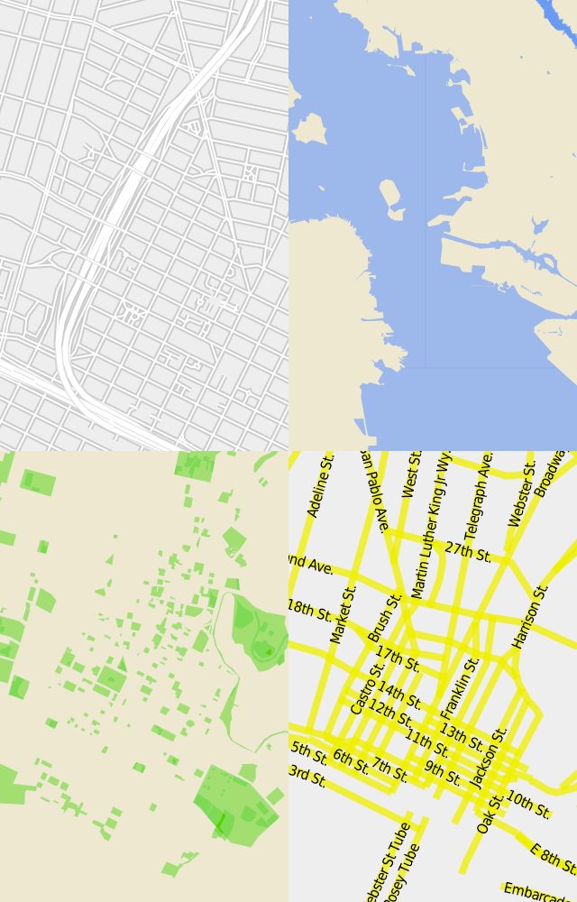
We just got new memory and faster storage on the OpenStreetMap US server, so I’m getting more comfortable talking about these as a proper service. Everything is available in TopoJSON and GeoJSON, rendering speeds are improving, and I’m adapting TopoJSON to Messagepack to support basic binary output (protobufs are a relative pain to create and use). I’m also starting to pay attention to the lower zoom levels, and adding support for Natural Earth data where applicable. So far, you’ll see that active in the Water and Land layers, with NE lakes, playas, parks and urban areas.
Last month, I followed up on Nelson Minar’s TopoJSON measurements from his State of the Map talk to make some predictions on the overall resource requirements for pre-rendering the earth. The remainder of this post is adapted from an email I sent to a small group of people collaborating on this effort.
Measuring Vector Tiles
I was interested to see how the vector tile rendering process performed in bulk, so I extracted a portion of the OSM + NE databases I’m using for the current vector tiles, and got to work on EC2. I found that render times for TopoJSON and GeoJSON “all” tiles were similar, and tile sizes for TopoJSON the usual ~40% smaller than GeoJSON.
What I most wanted from this was a sense of scope for pre-rendering worldwide vector tiles in order to run a more reliable service on the hardware we have.
I’m not thrilled with the results here; mostly they make me realize that to truly pre-render the world we’ll want to stop at ~Z13/14, and use the results of that process to generate the final JSON tiles sen by the outside world. This would actually be a similar process to that used by Mapbox, with the difference that Mapbox uses weirdly-formatted vector tiles to generate raster tiles, while I’m thinking to use weirdly-formatted vector tiles to generate other, less-weirdly formatted vector tiles. This is all getting into apply-for-a-grant territory, and I continue to be excited about the potential for running a reliable source of these tiles for client-side rendering experiments.
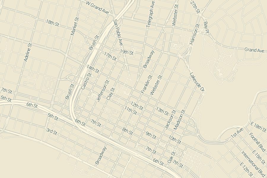
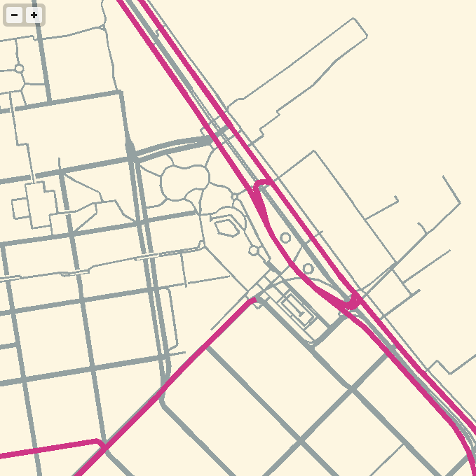
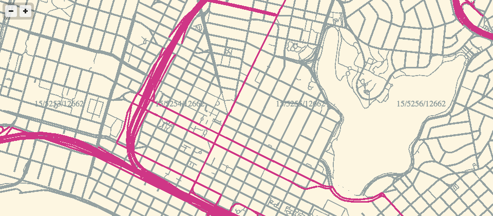
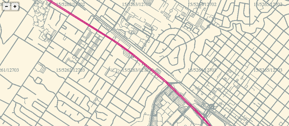
My area of interest is covered by this Z5 tile, including most of CA and NV: http://tile.openstreetmap.org/5/5/12.png
I used tilestache-seed to render tiles up to Z14, to fit everything into about a day. There ended up being about 350k tiles in that area, 0.1% of the total that Mapbox is rendering for the world. Since they I’m including several major cities, I’m guessing that a tile like 5/5/12 represents an above-average amount of data for vector tiles.
The PostGIS data was served from a 2GB database living on a ramfs volume, to mitigate EC2 IO impact.
Rendering Time
Times are generally comparable between the two, and I assume that it should be possible to beat some additional performance out of these with a compiled python module or node magic or… something. It will be interesting to profile the actual code at some point, I don’t know if we’re losing time converting from database WKB to shapely objects, gzipping to the cache, or if this is all good enough. Since our Z14s are not sufficient for rendering at higher zooms, I’ll want to mess with the queries to make something that could realistically be used to render full-resolution tiles from Z14 vector tiles.
The similar rendering times between the two surprised me; I expected to see more of a difference. I was also surprised to see the lower-zoom TopoJSON tiles come out faster. I suspect that with more geometry to encode at those levels, the relative advantage of integers over floats in JSON comes into play.
| Time | ||
|---|---|---|
| GeoJSON All | 4h31m | |
| TopoJSON All | 4h19m | 4% faster |
| Speed | ||
| GeoJSON Z14 | 2.67 /sec. | |
| TopoJSON Z14 | 1.71 /sec. | 36% slower |
| GeoJSON Z12 | 1.24 /sec. | |
| TopoJSON Z12 | 1.35 /sec. | 9% faster |
| GeoJSON Z10 | 0.23 /sec. | |
| TopoJSON Z10 | 0.25 /sec. | 9% faster |
Response Size
Nelson’s already done a bunch of this work, but it seemed worthwhile to measure this specific OSM-based datasource. TopoJSON saves more space at high zooms than low zooms. I measured the file length and disk usage of all cached tiles, which are stored gzipped and hopefully represent the actual size of a response over HTTP.
| Size (on disk) |
||||
|---|---|---|---|---|
| GeoJSON All | 2.1GB | |||
| TopoJSON All | 1.7GB | 19% smaller | ||
| Size (data) |
||||
| GeoJSON All | 922MB | |||
| TopoJSON All | 527MB | 43% smaller | ||
| Size (data) |
Tile (95th %) |
Tile (max) |
||
| GeoJSON Z14 | 673MB | 14.6KB | 135KB | |
| TopoJSON Z14 | 365MB | 46% smaller | 6.7KB | 75.2KB |
| GeoJSON Z13 | 165MB | 13.5KB | 176KB | |
| TopoJSON Z13 | 107MB | 35% smaller | 7.5KB | 112KB |
| GeoJSON Z12 | 62.9MB | 18.2KB | 106KB | |
| TopoJSON Z12 | 41.8MB | 33% smaller | 11.4KB | 80KB |
Jun 20, 2013 5:27am
disposable development boxes: linux containers on virtualbox
Hey look, a month went by and I stopped blogging because I have a new job. Great.
One of my responsibilities is keeping an eye on our sprawling Github account, currently at 326 repositories and 151 members. The current fellows are working on a huge number of projects and I frequently need to be able to quickly install, test and run projects with a weirdly-large variety of backend and server technologies. So, it’s become incredibly important to me to be able to rapidly spin up disposable Linux web servers to test with. Seth clued me in to Linux Containers (LXC) for this:
LXC provides operating system-level virtualization not via a full blown virtual machine, but rather provides a virtual environment that has its own process and network space. LXC relies on the Linux kernel cgroups functionality that became available in version 2.6.24, developed as part of LXC. … It is used by Heroku to provide separation between their “dynos.”
I use a Mac, so I’m running these under Virtualbox. I move around between a number of different networks, so each server container had to have a no-hassle network connection. I’m also impatient, so I really needed to be able to clone these in seconds and have them ready to use.
This is a guide for creating an Ubuntu Linux virtual machine under Virtualbox to host individual containers with simple two-way network connectivity. You’ll be able to clone a container with a single command, and connect to it using a simple <container>.local host name.
The Linux Host
First, download an Ubuntu ISO. I try to stick to the long-term support releases, so I’m using Ubuntu 12.04 here. Get a copy of Virtualbox, also free.
Create a new Virtualbox virtual machine to boot from the Ubuntu installation ISO. For a root volume, I selected the VDI format with a size of 32GB. The disk image will expand as it’s allocated, so it won’t take up all that space right away. I manually created three partitions on the volume:
- 4.0 GB ext4 primary.
- 512 MB swap, matching RAM size. Could use more.
- All remaining space btrfs, mounted at /var/lib/lxc.
Btrfs (B-tree file system, pronounced “Butter F S”, “Butterfuss”, “Better F S”, or “B-tree F S") is a GPL-licensed experimental copy-on-write file system. It will allow our cloned containers to occupy only as much disk space as is changed, which will decrease the overall file size of the virtual machine.
During the OS installation process, you’ll need to select a host name. I used “ubuntu-demo” for this demonstration.
Host Linux Networking
Boot into Linux. I started by installing some basics, for me: git, vim, tcsh, screen, htop, and etckeeper.
Set up /etc/network/interfaces with two bridges for eth0 and eth1, both DHCP. Note that eth0 and eth1 must be commented-out, as in this sample part of my /etc/network/interfaces:
## The primary network interface
#auto eth0
#iface eth0 inet dhcp

auto br0
iface br0 inet dhcp
        dns-nameservers 8.8.8.8
        bridge_ports eth0
        bridge_fd 0
        bridge_maxwait 0

auto br1
iface br1 inet dhcp
        bridge_ports eth1
        bridge_fd 0
        bridge_maxwait 0
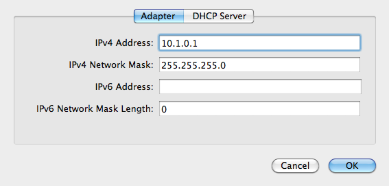
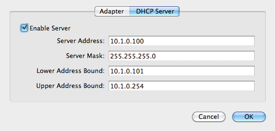
Back in Virtualbox preferencese, create a new network adapter and call it “vboxnet0”. My settings are 10.1.0.1, 255.255.255.0, with DHCP turned on.
Shut down the Linux host, and add the secondary interface in Virtual box. Choose host-only networking, the vboxnet0 adapter, and “Allow All” promiscuous mode so that the containers can see inbound network traffic.
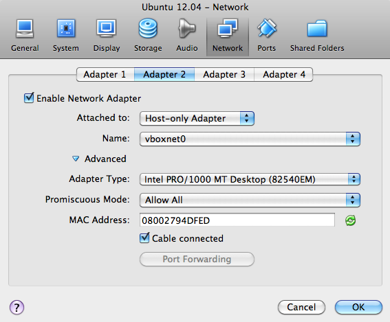
The primary interface will be NAT by default, which will carry normal out-bound internet traffic.
- Adapter 1: NAT (default)
- Adapter 2: Host-Only vboxnet0
Start up the Linux host again, and you should now be able to ping the outside world.
% ping 8.8.8.8

PING 8.8.8.8 (8.8.8.8) 56(84) bytes of data.
64 bytes from 8.8.8.8: icmp_req=1 ttl=63 time=340 ms
…
Use ifconfig to find your Linux IP address (mine is 10.1.0.2), and try ssh’ing to that address from your Mac command line with the username you chose during initial Ubuntu installation.
% ifconfig br1

br1       Link encap:Ethernet  HWaddr 08:00:27:94:df:ed
          inet addr:10.1.0.2  Bcast:10.1.0.255  Mask:255.255.255.0
          inet6 addr: …
Next, we’ll set up Avahi to broadcast host names so we don’t need to remember DHCP-assigned IP addresses. On the Linux host, install avahi-daemon:
% apt-get install avahi-daemon
In the configuration file /etc/avahi/avahi-daemon.conf, change these lines to clarify that our host names need only work on the second, host-only network adapter:
allow-interfaces=br1,eth1
deny-interfaces=br0,eth0,lxcbr0
Then restart Avahi.
% sudo service avahi-daemon restart
Now, you should be able to ping and ssh to ubuntu-demo.local from within the virtual machine and your Mac command line.
No Guest Containers
So far, we have a Linux virtual machine with a reliable two-way network connection that’s resilient to external network failures, available via a meaningful host name, and with a slightly funny disk setup. You could stop here, skipping the LXC steps and use Virtualbox’s built-in cloning functionality or something like Vagrant to set up fresh development environments. I’m going to keep going and set up LXC.
Linux Guest Containers
Install LXC.
% sudo apt-get lxc
Initial LXC setup uses templates, and on Ubuntu there are several useful ones that come with the package. You can find them under /usr/lib/lxc/templates; I have templates for ubuntu, fedora, debian, opensuse, and other popular Linux distributions. To create a new container called “base” use lxc-create with a chosen template.
% sudo lxc-create -n base -t ubuntu
This takes a few minutes, because it needs retrieve a bunch of packages for a minimal Ubuntu system. You’ll see this message at some point:
##
# The default user is 'ubuntu' with password 'ubuntu'!
# Use the 'sudo' command to run tasks as root in the container.
##
Without starting the container, modify its network adapters to match the two we set up earlier. Edit the top of /var/lib/lxc/base/config to look something like this:
lxc.network.type=veth
lxc.network.link=br0
lxc.network.flags=up
lxc.network.hwaddr = 00:16:3e:c2:9d:71

lxc.network.type=veth
lxc.network.link=br1
lxc.network.flags=up
lxc.network.hwaddr = 00:16:3e:c2:9d:72
An initial MAC address will be randomly generated for you under lxc.network.hwaddr, just make sure that the second one is different.
Modify the container’s network interfaces by editing /var/lib/lxc/base/rootfs/etc/network/interfaces (/var/lib/lxc/base/rootfs is the root filesystem of the new container) to look like this:
auto eth0
iface eth0 inet dhcp
        dns-nameservers 8.8.8.8

auto eth1
iface eth1 inet dhcp
Now your container knows about two network adapters, and they have been bridged to the Linux host OS virtual machine NAT and host-only adapters. Start your new container:
% sudo lxc-start -n base
You’ll see a normal Linux login screen at first, use the default username and password “ubuntu” and “ubuntu” from above. The system starts out with minimal packages. Install a few so you can get around, and include language-pack-en so you don’t get a bunch of annoying character set warnings:
% sudo apt-get install language-pack-en
% sudo apt-get install git vim tcsh screen htop etckeeper
% sudo apt-get install avahi-daemon
Make a similar change to the /etc/avahi/avahi-daemon.conf as above:
allow-interfaces=eth1
deny-interfaces=eth0
Shut down to return to the Linux host OS.
% sudo shutdown -h now
Now, restart the container with all the above modifications, in daemon mode.
% sudo lxc-start -d -n base
After it’s started up, you should be able to ping and ssh to base.local from your Linux host OS and your Mac.
% ssh ubuntu@base.local
Cloning a Container
Finally, we will clone the base container. If you’re curious about the effects of Btrfs, check the overall disk usage of the /var/lib/lxc volume where the containers are stored:
% df -h /var/lib/lxc

Filesystem      Size  Used Avail Use% Mounted on
/dev/sda3        28G  572M   26G   3% /var/lib/lxc
Clone the base container to a new one, called “clone”.
% sudo lxc-clone -o base -n clone
Look at the disk usage again, and you will see that it’s not grown by much.
% df -h /var/lib/lxc

Filesystem      Size  Used Avail Use% Mounted on
/dev/sda3        28G  573M   26G   3% /var/lib/lxc
If you actually look at the disk usage of the individual container directories, you’ll see that Btrfs is allowing 1.1GB of files to live in just 573MB of space, representing the repeating base files between the two containers.
% sudo du -sch /var/lib/lxc/*

560M	/var/lib/lxc/base
560M	/var/lib/lxc/clone
1.1G	total
You can now start the new clone container, connect to it and begin making changes.
% sudo lxc-start -d -n clone
% ssh ubuntu@clone.local
Conclusion
I have been using this setup for the past few weeks, currently with a half-dozen containers that I use for a variety of jobs: testing TileStache, installing Rails applications with RVM, serving Postgres data, and checking out new packages. One drawback that I have encountered is that as the disk image grows, my nightly time machine backups grow considerably. The Mac host OS can only see the Linux disk image as a single file.
On the other hand, having ready access to a variety of local Linux environments has been a boon to my ability to quickly try out ideas. Special thanks again to Seth for helping me work through some of the networking ugliness.
Further Reading
Tao of Mac has an article on a similar, but slightly different Virtualbox and LXC setup. They don’t include the promiscuous mode setting for the second network adapter, which I think is why they advise using Avahi and port forwarding to connect to the machine. I believe my way here might be easier.
Shift describes a Vagrant and LXC setup that skips Avahi and uses a plain hostnames for internal connectivity.
May 11, 2013 8:52pm
week 1,851: week one
I started my new gig this week, chief-technology-officering for Code For America. People have said nice things on Twitter, and I feel deeply welcomed.
I’ll write more about the actual thing soon, but for now I’m just basking in the weirdness of being in an office again. I have a desk and a calendar and colleagues and blooming, buzzing confusion. The code I’ve written this week is more angry, productive birds than TileStache or Extractotron, and that’s a funny feeling. There’s a shower at work, so I can ride my bike in and not offend people. The office is in SOMA, so I’ve started bringing my lunch. No one knew me when I was 25 (well, almost) and the organization is young, so the potential feels sky-high.
Soon, I will wear my new track jacket:

I’ve known Jen, Abhi, Meghan and the CfA team for many years, but I also spent most of April doing a big, serious grown-up job search. This was an entirely new experience for me, and very educational. I learned that recruiting is a real job for actual smart people at companies looking for talent, and that some people are mediocre at it while others are amazing. I learned that I enjoy technical interviews, the ones with whiteboards or pair-coding machines and one hour to solve a technical problem. Every single one that I did was fun, as long as I remembered to narrate my process and say “I don’t actually know what I’m doing here” where appropriate. I talked to some of the smartest, most interesting people I’ve ever dealt with and got to spend a whole month playing what-if with a variety of employers. I don’t know if this kind of abundance is something I’ll ever experience again, so I tried to savor it as much as possible.
Apr 22, 2013 6:30am
tilestache 0.7% better
TileStache, the map tile rendering server I’ve been working on since 2010, hit version 1.47 this weekend. The biggest change comes from Seth, who streamlined and expanded TileStache’s HTTP chops with the new TheTileLeftANote exception. The documentation needs an update, but the gist is that it’s now possible to customize tile HTTP responses from deep inside the rendering pipeline, with control over headers, status codes, and content. I’m excited that this didn’t require a backwards-incompatible change to the API, and that it’s now possible to tweak behavior in concert with Apache X-Sendfile or NGinx X-Accel.
Apr 10, 2013 10:45pm
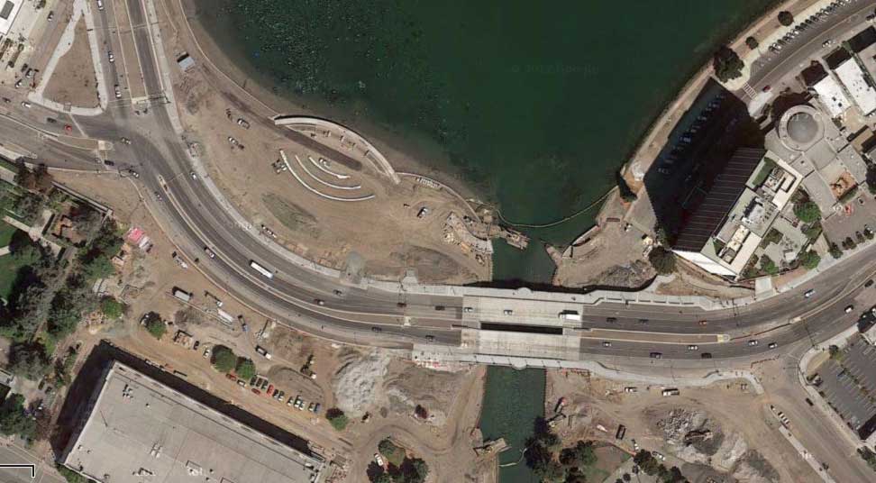
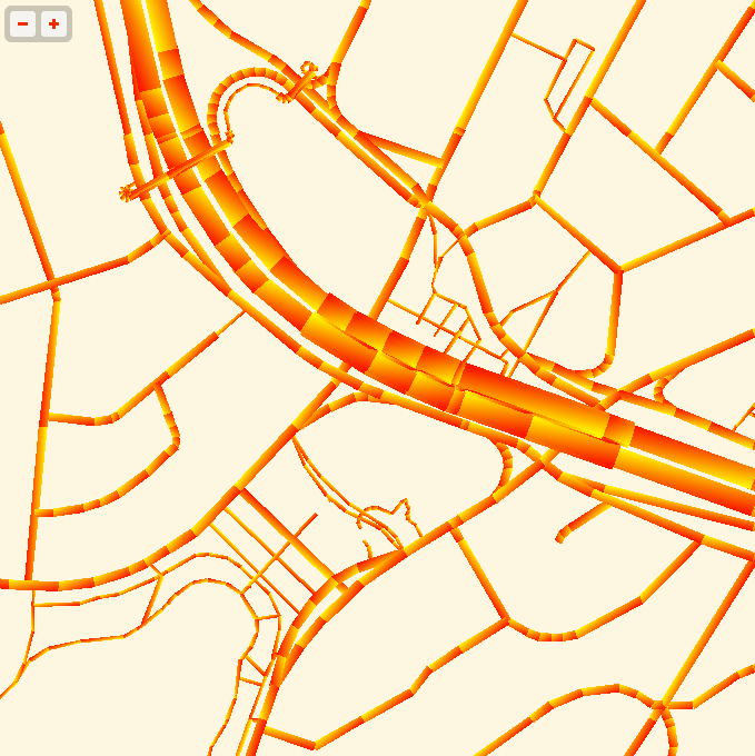
south end of lake merritt construction
Google Maps gives a nice unintentional before & after view of the construction along the south end of Lake Merritt in Oakland, if you turn the 45° aerials off and on.
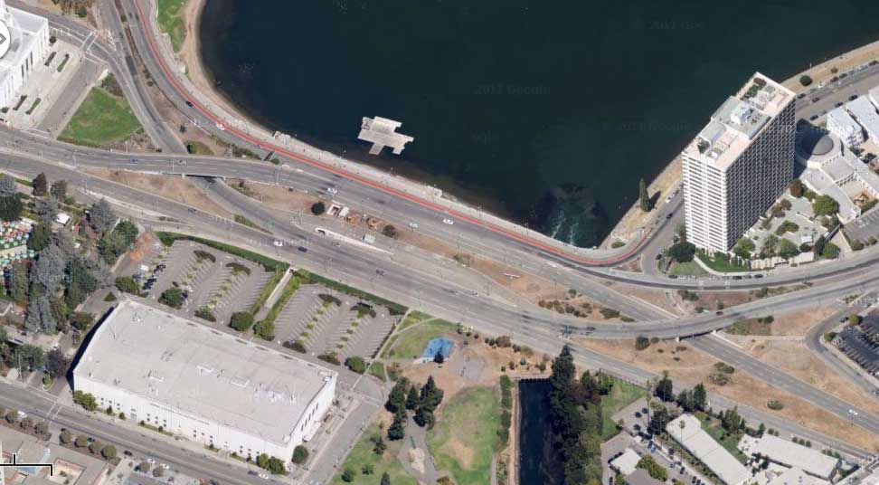
The gated-up and pissed-drenched pedestrian tunnels are gone. The connection to the bay is wider. There’s a separate pedestrian bridge, more grass, and proper crosswalks to the courthouse and museum.
Apr 6, 2013 2:44am
network time machine backups
I’ve been getting my house in order, computer-wise. I’ve maintained a continuous backup since Mac OS X introduced Time Machine several years ago, and I’ve grown increasingly uncomfortable with it just being a USB drive that I sometimes remember to attach when I’m at home. I researched network backups for the tiny home server (equivalent to a Raspberry Pi), and after struggling with a few of the steps I’ve got a basically-working encrypted backup RAID that runs transparently on my network and keeps my Mac OS X 10.6.8 Snow Leopard machine safe.
RAID
For durability, I wanted everything duplicated across two physical hard drives so that I could swap in new ones when failure made it necessary. RAID 1 is a standard for mirroring data to multiple redundant disks, and many manufacturers produce disk enclosures that do mirroring internally. I selected the NT2 from inXtron and two 2TB 3.5” hard drives, a total cost of ~$300.

The enclosure exposes a plain USB disk to Linux, identical to any other plug-in hard drive like the 2.5” one I was using previously. Unfortunately, the larger drives seem to require a fan in contrast to my previous silent drive. It’s not terribly loud, and a small price to pay for additional peace of mind.
udev
When connected, Linux assigns a drive letter to a USB volume, so that (for example) you can partition and mount from /dev/sda, /dev/sdb, etc. Unfortunately, these letters can be somewhat arbitrary, and you never know exactly where your connected drive will show up. This can be a real problem if you want the volume to be reliably findable every time. If you simply format the drive you can use the volume’s UUID instead of the drive letter, but I was interested in using Logical Volume Manager (LVM) so I needed it in a predictable place.
Fred Wenzel provided some hints on how to use udev, the device manager for the Linux kernel:
The solution for the crazily jumping dev nodes is the udev system, which is part of Linux for quite a while now, but I never really had a need to play with it yet. But the howto is pretty nice and easy to apply.
The idea is that you find some property of the device, like its manufacturer or product ID, and use that to create a stable link to the drive. With my drive temporarily at /dev/sda, I ran this udevadm command to read off its properties:
udevadm info -a -p /sys/block/sda/sda1
Running down the lengthy list that came back, I found three entries that looked meaningful:
ATTRS{manufacturer}=="inXtron, Inc."ATTRS{product}=="NT2"ATTRS{serial}=="0123456789"
This whole process was difficult and confusing, and I didn’t understand quite what I was doing until I started using udev’s PROGRAM/RUN functionality to log events and inspect them. I created a rule that matched all events with a “*”, and then had that log to a file in /tmp that I could periodically watch. It wasn’t necessary to reboot the server when testing, which was a big relief.
The rule I ended up with in /udev/rules.d/10-local.rules looks like this:
ATTRS{product}=="NT2", KERNEL=="sd*1", SYMLINK="raid"
It’s causes any one of /dev/sda1, /dev/sdb1, etc. with the product name “NT2” to be symlinked to /dev/raid. I could add the serial number, but this minimal rule works for now.
LVM
Logical Volume Manager makes it possible to do all kinds of neat tricks with hard drives, such as having a single volume span many physical disks or freely resize volumes and move them around after they are created. Setting up LVM requires three steps:
pvcreate /dev/raidto make a physical volume from /dev/raid.vgcreate lvmraid /dev/raidto create a new volume group called “lvmraid” from the /dev/raid physical disk.lvcreate -L 360g -n tmachine lvmraidto create a new 360GB logical volume at /dev/mapper/lvmraid-tmachine, which I want to use for my backup volume.
At this point, it would be possible to make a filesystem on /dev/mapper/lvmraid-tmachine and have a 360GB volume available. I’ve got more logical volumes than this, but I’m just showing the one.
Volume encryption
I wanted my backup to be safely encrypted, so I followed advice from Robin Bowes who shows how to use cryptsetup and Linux Unified Key Setup (LUKS):
cryptsetup -y --cipher aes-cbc-essiv:sha256 --key-size 256 luksFormat /dev/mapper/lvmraid-tmachinecryptsetup luksOpen /dev/mapper/lvmraid-tmachine lvbackupmkfs.ext3 -j -O ^ext_attr,^resize_inode /dev/mapper/lvbackup
The first step encrypts the volume, where you’ll assign a secret passphrase. The second step opens the volume at /dev/mapper/lvbackup, where you’ll have to provide the passphrase. The third creates a filesystem on the new volume; I’ve included some mkfs flags that omit features which might make it hard to resize the volume later.
I mount the new volume at /time-machine, and confirm that I can read and write files to it. I will need to run the luksOpen step every time I want to mount this volume after a reboot, so it’s useful to save a two-line script in /time-machine/mount.sh for reference.
Netatalk and AFPD
This was the second hard part; I’ve tried running Apple File exchange before and gave up, this time I figured out how to make it write meaningful logs so I could debug the process. The default installation of netatalk from apt-get mostly works, with a couple small changes:
- Add “-setuplog "CNID LOG_INFO" -setuplog "AFPDaemon LOG_INFO"” to afpd.conf, to watch CNID and AFPD log useful progress to /var/log/syslog.
- Replace the default uamlist in /etc/netatalk/afpd.conf, changing it from “uams_clrtxt.so,uams_dhx.so” to “uams_dhx2.so” so that Mac OS X can correctly provide a password. Until I did this, I was consistently seeing failed login attempts.
Finally, I added this line to /etc/netatalk/AppleVolumes.default:
/time-machine TimeMachine allow:migurski cnidscheme:cdb options:usedots,upriv
Now I have a working Apple File server.
Time Machine
Apple’s Time Machine is picky about the format of the volume it writes its backups to, preferring HFS+ to anything else. I initially looked at setting up /time-machine as an actual HFS volume, but stopped when I started reading words like “recompile” and “kernel”. Matthias Kretschmann offers a better way with Disk Utility. His netatalk advice is useful above, and I simply skipped all the Avahi steps. The important part of his article is under Configure Time Machine: ask Time Machine to show unsupported network volumes, and create your own sparsebundle disk image to back up to:
In short, you have to create the backup disk image on your Desktop and copy it to your mounted Time Machine volume. But Time Machine creates a unique filename for the disk image and we can find out this name with a little trick…
Actually follow his actual advice on the name of the file and volume, before copying to the AppleTalk share. My computer is named “Null Island”, so my sparse bundle file is called “Null-Island_xxxxxxxxxxxx.sparsebundle”. The x’s come from the hardware ethernet address, which you can find by running ifconfig en0 on the command line.
AutoBackup
Finally, in my case I don’t actually want Time Machine running at all hours of the day. When you switch to a network backup, everything takes longer than USB. I added these two lines to my crontab, causing AutoBackup to be kept off during the day, and kept on late at night:
*/5 23,0-8 * * * defaults write /Library/Preferences/com.apple.TimeMachine AutoBackup -bool true*/5 9-22 * * * defaults write /Library/Preferences/com.apple.TimeMachine AutoBackup -bool false
With this in place, I don’t saturate the network with backup traffic during the day, and I can guarantee that my data is safe by keeping the computer on overnight. Time Machine keeps Apple File credentials, so it’s capable of mounting the network drive on its own. I just need to have the computer on after 11pm and before 9am.
Apr 3, 2013 8:23pm
week 1,846: ladders
I finished Evgeny Morozov’s mega-screed The Meme Hustler (“Tim O’Reilly’s crazy talk”) yesterday. If you can squeeze uncomfortably past the acid-drenched ad hominem opener, Evgeny recounts the history of the Open Source vs. Free Software memetic war of the late 1990’s and its relationship to political power:
Ranking your purchases on Amazon or reporting spammy emails to Google are good examples of clever architectures of participation. Once Amazon and Google start learning from millions of users, they become “smarter” and more attractive to the original users. This is a very limited vision of participation. It amounts to no more than a simple feedback session with whoever is running the system. You are not participating in the design of that system, nor are you asked to comment on its future. There is nothing “collective” about such distributed intelligence; it’s just a bunch of individual users acting on their own and never experiencing any sense of solidarity or group belonging. Such “participation” has no political dimension; no power changes hands. … There’s a very explicit depoliticization of participation at work here.
This morning, Matt said this, in response to Wave’s comment/question about empowerment:
@drwave once you’re “there”: making sure you don’t pull up the ladder, making new, better ladders, admitting there was a ladder.
The image of the ladder sticks with me. I entered into awareness of Open-vs.-Free in 1999, when it looked like another Vi-vs.-Emacs thing, an interminable pissing match for nerds. In Morozov’s retelling, the power politics of Freedom and Openness look newly fresh, important all over again. It touches the question of who the ladder is for, who’s inside the tribe deserving of help, and how to think about equity. The Free Software side of the argument framed a bigger community, consisting of users and developers together. GNU's four freedoms name use and study before they name distribution and modification. Order matters, ladders are for everyone.
I spoke at Ragi Burhum’s Geomeetup yesterday, about my recent work on vector tiles for Mapnik. The slides are here in PDF form. One of the subtexts to my OSM work for the past few years has been the ladder-making that Matt describes: a way to make datasets like OSM available to more people who might not otherwise choose to learn the full set of tools needed to work with the raw stuff, but still have important things to say. That includes professional message-makers like journalists but also enthusiasts like Stephanie May or Burrito Justice (on tacos and history). There are commercial answers to this question from companies like Google or Mapbox, but in addition to those it should always be possible to take your message into your own hands, most especially if your message is likely to get under someone’s fingernails. Free software and free data work as one kind of ladder, continually looking back as well as forward, assimilating innovation and passing it down to where it wouldn’t otherwise reach. I’m tempted to call this “trickle down”, but it occurs to me that the pull of gravity is all wrong in that image. Things don’t move from the core to the gap like water flowing downhill, but quite the opposite. Left alone, innovation and capital accrue to where they are already in highest concentration. Collective work and effort are the only forces that can counteract gravity with any regularity.
Here is the data. Please tell me if you find it interesting, useful, or need help.
Mar 16, 2013 3:24am
documentation for tiled vectors in mapnik
I’ve documented the tiled MVT layers on offer (currently two), possibly underexplained yesterday.

Mar 15, 2013 6:09am
the liberty of postgreslessness: tiled vectors in mapnik
(tl;dr: VecTiles)
Data is one of OpenStreetMap’s biggest pain points. The latest planet file is 27GB, and getting OSM into the Postgres database can be a long and winding road.
Vectored tiles offer a way forward, and Mapnik is growing features to support them. Matthew Kenny writes about them on his blog from a Polymaps-like in-browser rendering angle, but I’m also thinking about how vectors could be used with Mapnik directly to render bitmaps without needing direct access to a spatial database.
Three parts are needed for this to work:
- A server with data that can render vector tiles.
- A datasource for Mapnik to request and assemble tiles.
- A file format to tie them together.
MVT (Mapnik Vector Tiles) is my first attempt at a sensible file format. In Polymaps and my WebGL mapping experiments I’ve been using GeoJSON, but it has a few disadvantages for use in Mapnik.
One problem that GeoJSON doesn’t suffer from is size: when simplified at the database level, truncated to six digits of floating point precision at the JSON encoding level and gzipped at the HTTP/application level GeoJSON shrinks surprisingly well. At zoom level 14, the data tiles for San Francisco’s artisinal hipster district take up almost 700KB, but gzip down to just 45KB. At zoom level 16, those same data tiles require 1.16MB but gzip down to 76KB. That’s a crazy 94% drop in size on the wire, not out of line with what I’ve been seeing in practice.
GeoJSON’s big disadvantage is the reëncoding work necessary at the client and server ends. Shapely offers quick convenience functions for converting to and from GeoJSON, but you’re still spending cycles reprojecting between geographic and mercator coordinates, and parsing large slugs of GeoJSON is needlessly slow.
Since Mapnik 2.1, there has been a Python Datasource plugin that allows you to write data sources in the Python programming language, and it wants its data as pairs of WKB and simple dictionaries of feature properties. MVT keeps its data in binary format from end-to-end and never leaves the spherical mercator projection, so most of the data-shuffling overhead is skipped entirely. MVT uses zlib internally to compress data, and I reduce the floating point precision of all geometries using approximate_wkb to make them more shrinkable.
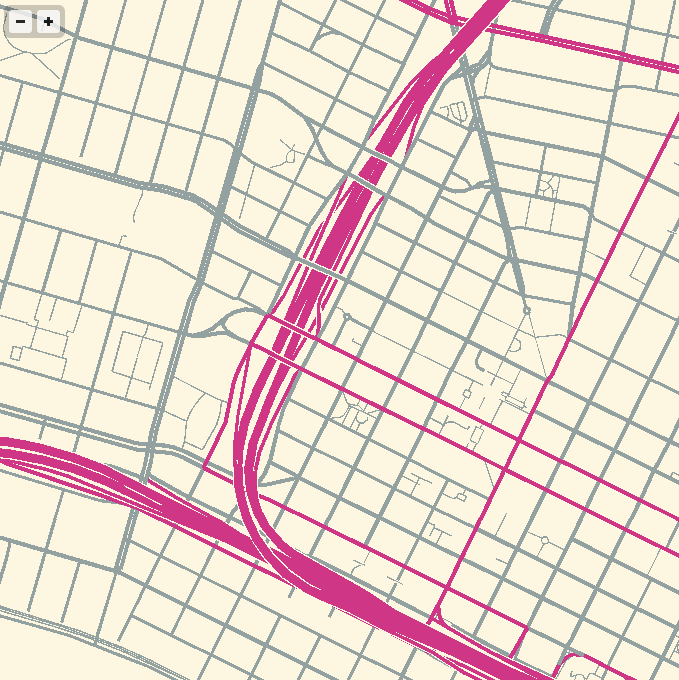
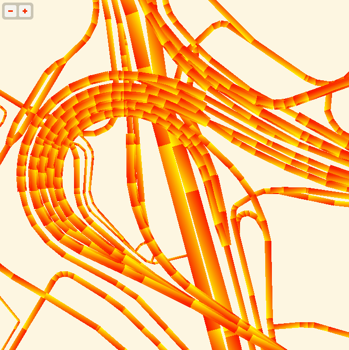
The performance I’ve seen has been decent, all things considered. This map of downtown Oakland rendered in 1.5 seconds, and two-thirds of that time was spent waiting on network latency:

On the server side, I’m using the new TileStache VecTiles.Provider to generate tiles. It makes both GeoJSON and MVT. It’s been especially interesting thinking through “where” cartography lives in a setup like this. I spoke with Dennis McClendon when I visited Chicago recently, and he pointed out how there’s now a divide between data and rendering in digital cartography that doesn’t exist for him. Traditionally, making a map meant collecting and curating data. Only with the distributed labor force of the OpenStreetMap community and the effort of projects like Mapnik can you frame cartography separately from data. Vector tiles blur this distinction somewhat, because the increased distance and narrower bandwidth between renderer and data source forces some visual decisions to be made at the data level. Tiles for drawing lines vs. labels, for example, are separate: lines can be clipped at tile edges and flags for bridges, tunnels and physical layering must be preserved, while labels demand unclipped geometries and simpler lines.
A portion of the live TileStache configuration looks like this, with linked Postgres queries.
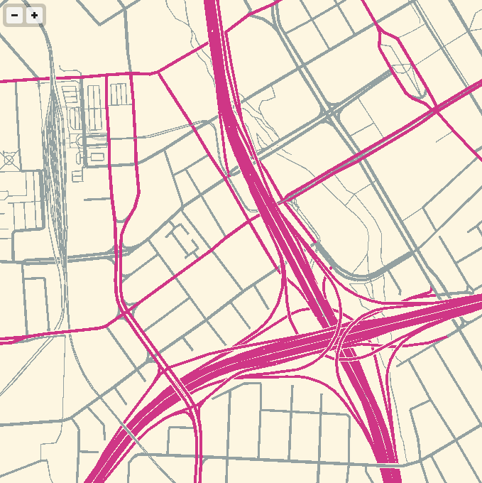
The division of linework and labels into separate layers yields this rendering at zoom 15, completed in 2.7 seconds with about 1.1 seconds of network overhead:
Back on the client side, the TileStache VecTiles.Datasource provides data retrieval, sorting and rendering capability to Mapnik. I’ve tested it with Mapnik XML stylesheets, Carto on the command line and Cascadenik and it’s worked flawlessly everywhere. I’ve not tried it with Tile Mill. The project MML file contains simple URL templates in the datasource configuration, while the style MSS is essentially unchanged from a typical Mapnik project.
The Mapnik Python Datasource API expects data in the projection of the final rendering, delivered as WKB geometry and simple dictionaries with strings for keys (not unicode objects, a Mapnik gotcha). Inside the zlib-compressed payload of an MVT tile, this data is provided almost without change. For unclipped geometries, unique values are determined by value using the whole of the WKB representation, and there’s not a point anywhere in the client process where the WKB is decoded or parsed until it hits Mapnik.
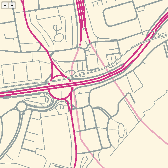
This zoom 13 rendering still demands 1.1 seconds of network overhead, plus 2.7 seconds of actual CPU work to render all the small streets:
I suspect that the network overhead would drop substantially if I allowed the client Datasource to request much larger tiles, either 512×512 or 1024×1024 at a time instead of the traditional 256×256. This is quite easy to do in code but the expectations around line simplification and correct behavior at each zoom level are challenging. I’m struggling to find the balance here between my own fluency in tile coordinates and something trivially usable by cartographers and Tile Mill users hoping to skip the database grind.
Doing this all over HTTP has huge advantages, despite the network overhead. For example, the tiles used in the examples above are all requested from tile.openstreetmap.us, which happens to make use of Fastly’s caching CDN to ease traffic load on the OSM-US server. Running your own caching proxy to bring it all closer seems more trivial than learning how to set up Postgres.
Overall, I think VecTiles and MVT offer a compelling way to use Mapnik or Tile Mill with no local datastore. The test tiles I’m working with are served from OSM-US Foundation supported hardware, where Ian Dees and others have ensured an up-to-date database. It should be possible to take advantage of OpenStreetMap for cartography without learning to be a database hero.
Since you’ve read this far, here’s the Mario Kart Rainbow Road edition of WebGL maps that uses these tiles:

Feb 28, 2013 12:03am
gl-solar, webGL rendering of OSM data
I’ve been experimenting with WebGL rendering of vector tiles from OpenStreetMap, and the results so far have been quite good.
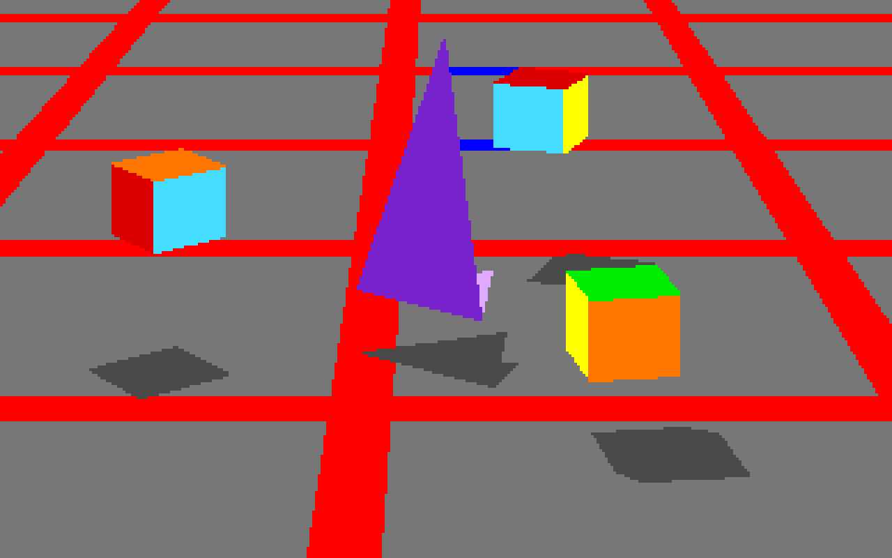
Techniques for fast, in-browser drawing of street centerlines have interested me since I looked closely at the new iOS Google Maps, which uses vector rendering to achieve good-looking maps on the small screen of a phone.
While Google seems to have aimed for an exact duplicate of their high-quality raster cartography in a more interactive package, I’ve been playing with the visual aesthetics of aliased edges and single, flat expanses of color. The jaggies along the edge of Facebook’s parking lot in the screen above remind me of early 1990s side-by-side print quality comparisons from Macworld, except I always preferred the digitally-butchered woodcut edges in the 200dpi samples to the too-perfect reproduction in the 600dpi+ version. At the very moment that they’re disappearing into a retinal haze, pixels are looking good again.
The colors here are all transposed from OSM-Solar, my cartographic application of Ethan Schoonover’s Solarized, a sixteen color palette (eight monotones, eight accent colors) designed for use with terminal and gui applications.
For the depth-sorting of roads and correct display of under- and overpasses, I’m using the “layer” metadata found in some OSM objects and my own High Road OSM queries. WebGL is amazing for this, because all the actual sorting is happening in the vertex shader where it can happen quickly and in parallel.
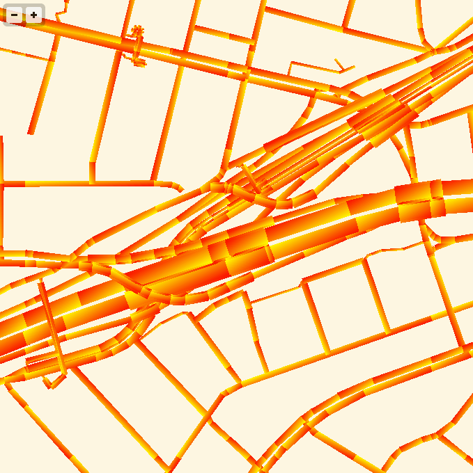
The road widths are being calculated manually, based on simplified centerline geometries found in GeoJSON tiles. I’m inflating each road type by a variable amount, manually creating my own line joins and caps. The image above is from the false color edition, which shows much more clearly how the line widths are being constructed. Javascript is reasonably fast at this basic trigonometry, but I had to move this part of the code into a web worker to cut down on animation glitches.
The panning and zooming smoothness are astonishing; overall I’ve been very happy with performance. One challenge that I’d like to address is the breakdown in floating point precision at zoom level 18. Four-byte floats have a 24-bit significand, which allows for pixel-perfection only up to zoom level 16 on a world map. The effect is relatively subtle at zoom 17, but glaringly obvious and a big problem at 18. I like the visual appearance of the aliased lines, but they wouldn’t be appropriate for everyday use of a map.
I imagine at some point I will need to add buildings, water and labels. One step at a time. The code for this demo is available on Github, and the correct link for the demo itself is http://teczno.com/squares/GL-Solar/.
More sample screen shots below.


Feb 26, 2013 9:34am
webgl maps, stealth mountain edition
More about these later, but for the moment I am just loving the aliased aesthetic of pure-webGL OSM renderings.
If the color scheme looks familiar, it’s because I’ve worked with it before.
Feb 19, 2013 4:58pm
one more (map of lake merritt)
Lake Merritt is the Lenna of cartography samples. Here’s one more from Ars Technica:

—Cyrus Farivar in Ars Technica, Hands-on with RunKeeper 3 for iPhone.
Feb 19, 2013 7:44am
elephant-to-elephant: processing OSM data in hadoop
Usable line generalization for OSM roads and routes has been a hobby project of mine for several years now, since I argued for it at the first U.S. State of the Map conference in Atlanta, 2010. I’ve finally put the last piece of this project in place with the use of Hadoop to parallelize the geometry processing.
I’ve learned a lot about moving geographic data between Postgres and Hadoop. The result is available at Streets and Routes.

Matt Biddulph gave me a brief introduction to using Hadoop’s streaming utility, the summary of which was that it’s just a reasonably-smart manager of scripts that push text at each other:
The utility allows you to create and run Map/Reduce jobs with any executable or script as the mapper and/or the reducer. …both the mapper and the reducer are executables that read the input from stdin (line by line) and emit the output to stdout. The utility will create a Map/Reduce job, submit the job to an appropriate cluster, and monitor the progress of the job until it completes.
(MapReduce is Google’s 2004 data processing approach for big clusters)
I’d been building something like it myself, so it was a relief to dump everything and switch to Hadoop. Amazon’s Hadoop distribution, known as Elastic MapReduce, offers an additional layer of management, handling the setup and teardown of machines for you. Communication generally happens via S3, where you load your data and scripts and pick up your results. On the EC2 side, Amazon tends to use recent versions of Debian Linux 6.0, which means that all the nice geospatial packages you’d expect from apt are available.
Easy.
For this project, I’ve added Hadoop scripts directly to Skeletron, my line-generalization tool. There’s a mapper and a reducer. Everything speaks GeoJSON because it’s easy to parse in Python and use with Shapely. If you’re familiar with pipes in Unix, the entire process is exactly equivalent to this, spread out over many machines:
cat input | mapper | sort | reducer > output
The only tricky part is in the middle, because Hadoop’s sorting and distribution of the mapped output expects single lines of text with a tab-delimited key at the beginning. In Skeletron, I created a pair of functions that convert geographic features to text (base64-encoded Well-Known Binary) and back. Only the mapper’s input and reducer’s output need to speak and understand GeoJSON. Hadoop is pretty smart about the data it reads, as well. If you tell it to look in a directory on S3 for input and it finds a bunch of objects whose names end with “.bz2,” it will transparently decompress those for you before streaming them to a mapper.
So, the process of moving data from a PostGIS table created by osm2pgsql through Hadoop takes five steps:
- Dump your geographic data into GeoJSON files.
- Compress them and upload them to a directory on S3.
- Run a MapReduce job that accepts and outputs GeoJSON data.
- Wait.
- Pick up resulting GeoJSON from another S3 directory.
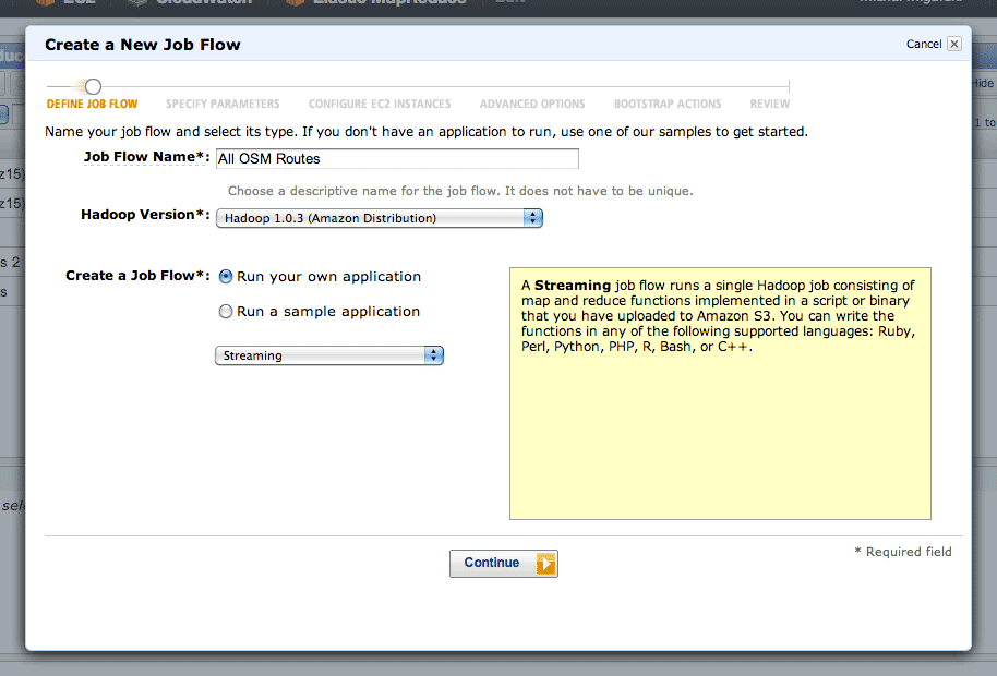
Running a MapReduce job is mostly a point-and-click affair.
After clicking the “Create New Job Flow” button from the AWS console, select the Streaming flow:
The second step is where you define your inputs, outputs, mappers and reducers:
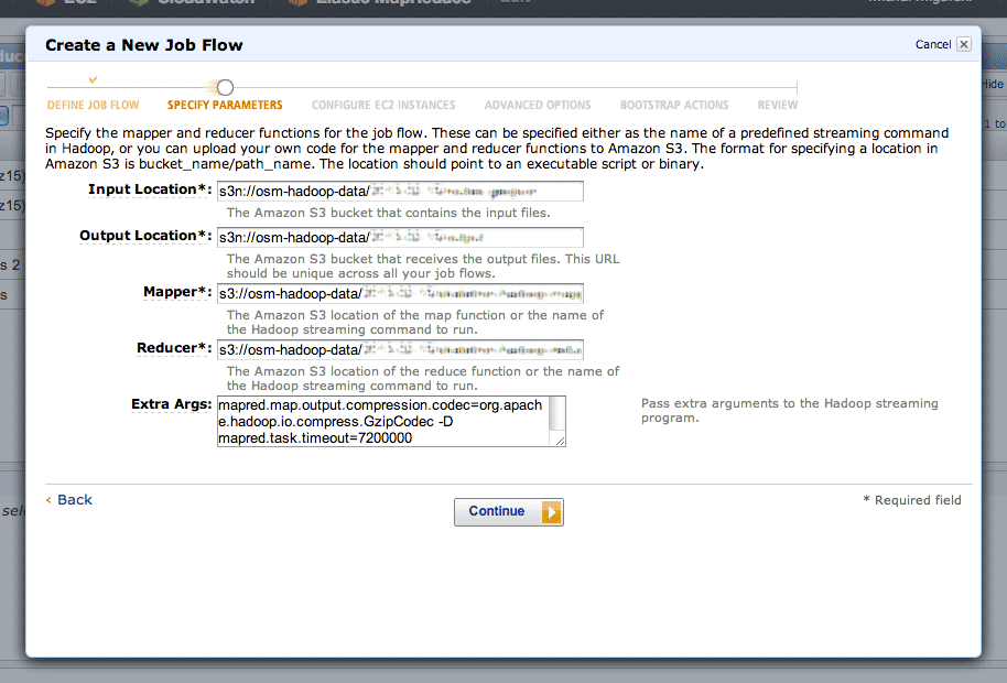
The “s3n:” protocol is used to refer to directories on S3, and the “osm-hadoop-data” part in the examples above is my bucket. For the mapper and reducer, I’ve uploaded the scripts directly from Skeletron so that EMR can find them.
The extra arguments I’ve used are:
- -D mapred.task.timeout=21600000 to give each map task six hours without Hadoop flagging it as failed. By default, Hadoop assumes that a task will take five minutes, but some of the more complex geometry tasks can take hours.
- -D mapred.compress.map.output=true to compress the data moving between the mappers and reducers, because it’s large and repetitive. The compression codec is given by -D mapred.map.output.compression.codec=org.apache.hadoop.io.compress.GzipCodec.
- -D mapred.output.compress=true to compress the output data sent to S3. The compression codec is given by -D mapred.output.compression.codec=org.apache.hadoop.io.compress.BZip2Codec.
Step three is where you choose your EC2 machines. Amazon’s spot pricing is a smart thing to use here. I’ve typically seen prices on the order of $0.01 per CPU-hour, a huge savings on EC2’s normal pricing. Using the spot market will introduce some lag time to your job, since Amazon assumes you are a flexible cheapskate. I’ve typically experienced about ten minutes from creating a job to seeing it run.
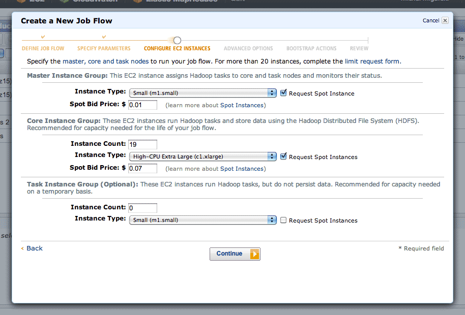
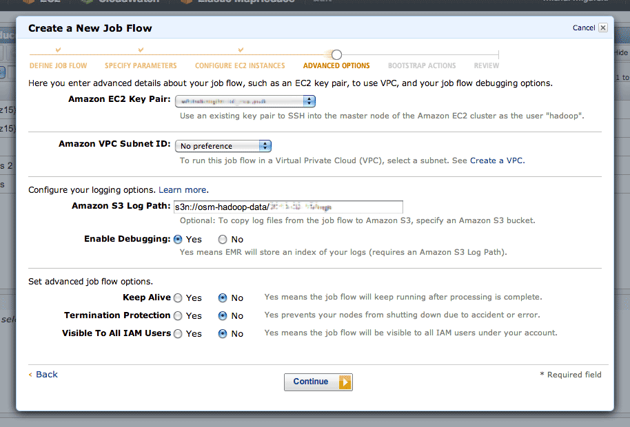
In step four, there are two interesting advanced options. Setting a log path will get you a directory full of detailed job logs, useful when something is mysteriously failing. Setting a key pair will allow you to SSH into your master instance, which runs a detailed Hadoop job tracker UI over HTTP on port 9100 (SSH tunnel in to see it in a browser). The tracker lets you dig into individual tasks or see an overall progress graph.
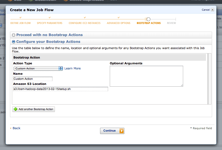
Step five is where you can define a setup script. This script is where you’ll do all of your per-machine preparation, such as downloading uniform data or installing additional packages.
For lengthy jobs, EMR’s graphs are a useful way to observe job flow progress. Your two most useful graphs are Average Map Tasks Running (top left), telling you how many mapper tasks are currently in progress, and Average Map Tasks Remaining (second from left on the top row), telling you how many mapper tasks have not yet started.
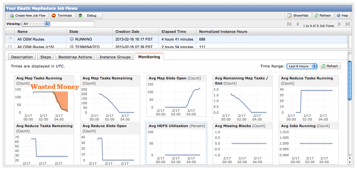
While the job is in progress, you’ll see the second graph progress downward toward zero, and the first graph pegged to the top and then progressing downward as well. The amount of time the first graph spends below the maximum represents wasted money, spent on CPU’s twiddling their thumbs waiting for straggler jobs to come in. This problem will be worse if you have more machines working on your job, leading to a very simple speed/cost tradeoff. If you want your job done fast, some of your machines won’t be doing much once the main crush is over. If you want your job done cheap, keep a smaller number of machines going to reduce the number of idle processors at the end.
I ran the same job twice with a different number of machines each time, and saw a cost of $4.90 for five instances over 17 hours vs. $9.40 for twenty instances over 7 hours. If you don’t need the results fast, save the five bucks and let it run overnight. If you don’t use spot pricing, this same job would have cost $40 slow or $78 fast.
To try all this yourself, I’ve set up a bucket with sample data from the OSM route relations job.
The end result is something I’m super happy about: a complete worldwide dataset of simplified roads and routes that’s suitable for high-quality labels and route shields.
Feb 16, 2013 8:31am
beasts of the southern wild
We saw Beasts of the Southern Wild yesterday, still thinking about it today. It’s a beautiful, surrealist, magical realist story about a hurricane evacuation south of New Orleans. Everything is told through the eyes of a six year old, whose acceptance of the facts of nature around shocked me, one after another. All animals are made out of meat. Prehistoric aurochs thawing from the arctic ice and floating down to the Gulf of Mexico. Streams of gorgeous, post-apocalyptic imagery. Perfect acting by Dwight Henry.

Feb 12, 2013 11:00pm
weeks 1,838/1,839: total protonic reversal
On an airplane coming back from Washington, DC. I’m trying to be good at this weeknotes thing, but I’m also somewhat speechless for the moment so this will be short.
Code is a thing I can talk about most comfortably in the context of a weeknote, otherwise it turns into strangely unsatisfying codename mystery project blogging.
I’ve formalized last week’s Typescript experiment into a standalone map tile library called Squares. A demo that loosely duplicates the recently-departed getlatlon.com shows what it’s generally capable of, which at the moment is Not A Ton. I think the Typescript experiment feels like a success, and I’m starting to point Squares at other projects that have been waiting for it to take shape.
When I wasn’t hacking at Typescript last week, I was at an actual desk working with Trifacta in San Francisco on data and UX consulting.
We also had a record nine people at our weekly geogeek breakfast at the Mission Pork Store, up from a typical five or six. Onward.
While in DC, I fully caught up with Team Mapbox and batted around some OpenStreetMap US 2013 ideas with Eric, Alex, Tom, and Bonnie. We watched Ted, the one about the talking bear, and drank cheap beer from cans.
This week, more of all that and talking and hopefully some new code and cartography finally.
Feb 4, 2013 1:38am
week 1,837: typescripting
This has been week six of self-exile and funemployment.
Since JS.Geo, I’ve been reflecting on the world-consuming popularity of Mike Bostock and Jason Davies’s D3 library and giving it a repeat test-drive. I think there are two fascinating aspects to the public response to D3 at events like JS.Geo: everyone wants to do something with it, but very few people claim to understand it. I attempted to explain the “.data()” method to a friend at JS.Geo and realized that I also was missing a critical piece myself. One metaphor I’ve been using to think about D3 has been performance: Mike and Jason are so deeply good at what they do and create such a prolific stream of examples that just watching the work is like a stage performance. They’re the current reigning Penn & Teller of Javascript, the Las Vegas tiger guys of SVG, and you can’t not be fascinated even as your watch disappears. The problem with this metaphor is that it puts up a wall between you and the code, frames it as an unobtainable skill. There’s not much you can learn about personal fitness from watching a professional dancer at work. So, performance is an unhelpful metaphor.
A more useful metaphor I’ve been exploring in code this week is D3 as nuclear fuel. This starts to feel a bit more helpful, because it suggests a clear approach to D3 for mortal developers: use the power, but keep it carefully contained. It’s the same line of thinking suggested by Rebecca Murphey’s argument about jQuery: “it turns out jQuery’s DOM-centric patterns are a fairly terrible way to think about applications,” leading to Tom Hughes-Croucher’s idea of pyramid code, “huge chains of nested, dependent anonymous callbacks piled one on top of another.” With great power comes great blah blah blah. Observing Dr. Manhattan offers little guidance for building a power plant.

I’ve always enjoyed strongly-typed languages for interactive work, so this week I have been approaching the use of D3 from the direction of Typescript, Microsoft’s typed superset of JavaScript that compiles to plain JavaScript. The Typescript team have helpfully created a starting set of declarations for D3, making it possible to use the relatively-structureless method chains within a more controlled environment.
I’m surprised at how much I enjoyed Typescript, and how comfortable it felt immediately, and how fun it’s been to bounce a free-form library like D3 against a strictly-typed language environment, like a super ball off a concrete wall. My test project is a fork of Tom Carden’s D3Map, an exercise in learning D3 for DOM manipulation and transitions. Play with it live at bl.ocks.org/4703593. You can use Typescript to write legible, self-describing code with clearly enforced expectations like Grid.ts. You can also keep the D3-needing parts carefully separated from the tile math like Image.ts and Mouse.ts. The additional structure demanded by Typescript felt surprising calming, like Allen Short’s 2010 PyCon talk on Big Brother’s Design Rules (via War is Peace):
- Slavery is Freedom: the more you constrain your code's behavior, the more freedom you have to act.
- Ignorance is Strength: the less your code knows about, the fewer things it can break. This is itself a play on the Law of Demeter or principle of least knowledge.
The one major bump I experienced with Typescript was in deploying to a browser. Although Typescript files compile to Javascript, they include calls to “require(),” a part of the CommonJS spec. This is not browser-kosher, so I used Browserify in the Makefile to generate a browser-compatible file with an extra 9KB slug of CommonJS overhead.
All of this has been a step on the way to a browsable WebGL map, one of my goals from last week.
I have also significantly updated the visual appearance of Green Means Go to make it more legible and hopefully printable.
No current progress on Metro Extracts.
This week, I’ll be doing some consulting and some future conspiracy planning. People will be visiting town, and I will have beers with them.
Jan 23, 2013 1:55am
week 1,836: back at shiny
Last week I announced my departure and many friends said nice, encouraging things on Twitter and here. Thank you. I’m sort of leaping into the abyss here, and it makes a huge difference to know I’m not just twisting in the wind.
Chicago and Denver were both cold and fun. I attended Chris Helm, Steve Citron-Pousty and Brian Timoney’s event JS.Geo. Peter Batty has a complete writeup, which doesn’t quite do justice to the absolute ubiquity of D3 at the conference. It was a good opportunity for me to finally/again get my head straight with D3 data joins with Seth and Aaron Ogle. I remain convinced that as D3’s primary feature, this is sadly under-documented. In Denver, my mustache repeatedly iced over. In Chicago, less so but it was still pretty cold.

I’m back now, and picking up a few projects.
Green Means Go is due for some thinking about individual counties. I’d like to create a single, printable view for each of 3000+ counties with some information about OSM coverage attached.
I’m starting to look at tiled data, D3 and WebGL together for the Nokia WebGL Maps. I’m super excited about the possibilities of shaders here, and need to get my head around tile-like loading of linear ArrayBuffers.
The Metro Extracts are overdue for an update, and I’d like to start doing these more regularly using OSM-US Foundation hardware. Some recent interest in the project suggests that I’ve been paying too little attention to it.
Some small potential consulting gigs, and general future planning.


Jan 15, 2013 7:34am
week 1,835: leaving stamen

I am in Denver. Wednesday I will be in Chicago. Friday night I will be back in Oakland. Here, I am visiting JS.Geo conference catching up on all the Javascript map-making I’ve missed over the years. In Chicago, I hope to meet with folks from the campaign now that it’s all over, and some new people.

On the last day of Baktun 13 of the Classical Mayan calendar, we held our annual holiday party. The next morning, we pushed the couches into the big room with the projector, screen and speakers, and spent most of a workday watching season three of Arrested Development and snacking on popcorn and lunch from Pancho Villa. It was the last day of the year, and my final day at Stamen.

Leaving is difficult. I’ve worked with Stamen and Eric Rodenbeck in particular for nine years. I’m sad to not be able to spend much time with new Stamens Mike Tahani and Beth Schechter, and I’m over the moon that Eric and Shawn have brought on Seth Fitzsimmons as my successor. Seth’s worked with us on projects in the past, knows us from the old office, and will fit right in.
In retrospect I’m shocked at how young I was when I joined. I’ve learned firsthand how a world-class design studio is run from one of the best creative directors in the industry, instigated, participated in or merely watched innumerable high-profile public research and client projects, and I’m proud to have seen us grow to a position of prominence and respect in the public’s perception of art and data. The work has never not been good, and my colleagues from over the years are some of my closest friends.

Still, nine years is a long-ass time.
It was like graduate school, art school, and business school all rolled into one and I feel ready to explore in some new directions. For the moment, that means catching up on things: sleep, books, hacking and design projects, exercise, regular blogging, and more. Soon, it will mean looking at new possibilities. For the moment, I don’t know what awaits me in the after but if you’re up for lunch I’m probably game.

Jan 9, 2013 2:55am
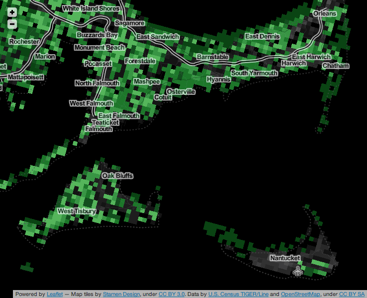
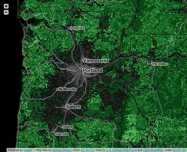
work in progress: green means go
Since State Of The Map in Portland, I’ve been applying simple raster methods to OpenStreetMap data to draw a picture of the current state of U.S. Government TIGER/Line data in the project. TIGER data is a street-level dataset of widely varying quality covering the whole of the United States, and much of OSM in this country is built on TIGER. OSM US Board member Martijn Van Exel explains, in his TIGER deserts post:
Back in 2007, we imported TIGER/Line data from the U.S. Census into OpenStreetMap. TIGER/Line was and is pretty crappy geodata, never meant to make pretty maps with, let alone do frivolous things like routing. But we did it anyway, because it gave us more or less complete base data for the U.S. to work with. …there’s lots of places where we haven’t been taking as good care of the data. Vast expanses of U.S. territory where the majority of the data in OSM is still TIGER as it was imported all those years ago. The TIGER deserts.
TIGER data has been a fantastic leg up for the U.S. map, but elsewhere in the world data imports are frowned upon. The german community in particular feels that imports are antithetical to local community mapping. The U.S. is very different from Europe in terms of population density and driving distances. As Toby Murray said in this message last year, the imbalance between mapper population and surface area between Kansas and Germany is potentially insurmountable:
It is a 9 hour drive from Topeka to Denver and I think you go past a total of 3 cities with a population of over 10,000. In fact, out of the 54 counties west of Wichita, only 7 have a population for the whole county of over 10,000. So while we might be able to start OSM communities in some of the larger cities, vast stretches of the country would remain completely empty.
In many rural parts of the country, the prospective local OSM mapping population and the creators of government data are exactly the same people. I talked to an Esri employee at SOTM this year who told me that at every year's User Conference, she gets a regular stream of these folks approaching her with data in hand, asking how they can get it into OSM. They are the local community we want, and it’s not always clear how we can help them help us.
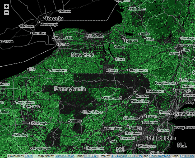
Based on the full history dump, I’ve been working on a map that I’m calling “Green Means Go,” a visualization of the state of TIGER/Line data in OpenStreetMap. The map shows a grid of 1km×1km squares covering the continental United States. Green squares show places where data imports are unlikely to interfere with community mapping, based on a count of unique participating mappers who don’t appear to be part of any of the three big TIGER imports.
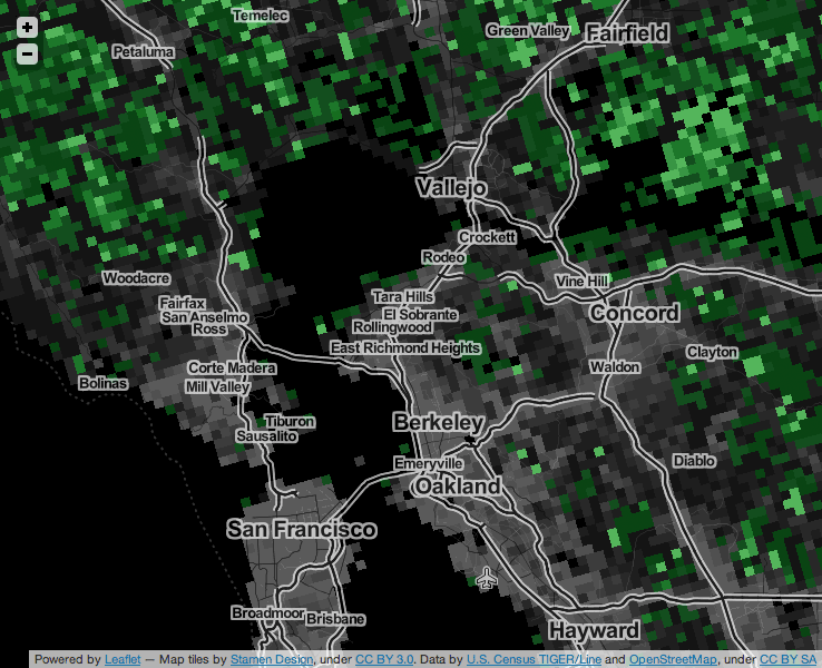
Large, densely-populated urban areas show a similar pattern, with a dark center where many individual mappers have contributed, surrounded by a green rural fringe where no OSM community members have participated in the cleanup and checking of TIGER data.
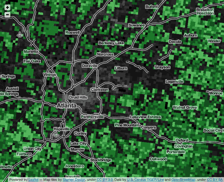
This pattern shows a lot of local variety. For example, the area around Portland and Salem in Oregon, where we held last year’s SOTM-US conference, shows a broad swath of edited area. Portland in particular has shown a strong local uptake of OSM, basing its official TriMet trip planner on OpenStreetMap.
Other parts of the country, especially in the Great Plains, show the pattern of relative non-participation described by Toby Murray:

Good data does exist in these places, and in fact can be found in the more recent TIGER data sets which rely much more heavily on data generated directly by local county officials. In an area like the one above, the Green Means Go map should help a GIS data owner see that his or her own data and local knowledge would interfere minimally (if at all) with local community mappers.
In some cases, we see patterns that are worth exploring further. Entire counties in Pennsylvania show up as edited, but it’s not obvious to me that there is a county-wide local community here. Have these areas already been replaced by county-level importers who’ve improved the data, or is there some portion of the 2007 TIGER import that I’m missing?
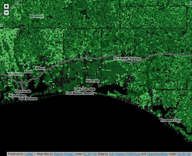
In this other image, the relative lack of any kind of data (OSM or TIGER) is visible on the grounds of Eglin Air Force Base, south of Interstate 10 and east of Pensacola in Florida:
This work is heavily in progress. I’d also like to write about the process of making it, using the National Landcover Dataset and Hadoop to generate this imagery. Some possible next steps include:
- Collaborating with Ian Dees, Alex Barth, Ruben Mendoza and others from the US OSM community to develop better ways of seeing TIGER data.
- Creating static, per-County and Census Place views.
- Developing a plan to regenerate these map tiles for future data updates.
Jan 7, 2013 12:31am
loading artifacts, google maps for iOS
The new GMaps for iOS uses the same/similar vector loading process as its longtime Android counterpart. The high-res stuff, including buildings and tiny streets, looks like it comes in right at zoom level 16, which is about where I would’ve put it given the choice.


The transition between zooms is a bit odd. I would not have expected the difference in street widths between the loaded and unloaded sections here. OpenGL does how (as far as I know) have its own concepts like round line caps or joins, so maybe there’s some client-side buffering these that’s expensive to run more than once per geometry load? The “hot dog” street endings show that each tile’s worth of geometry data comes clipped; I haven’t tested to see whether street names straddle z16 tile boundaries or not.


Interestingly, GMaps makes no attempt to model elevated freeways, terrain, or anything else vertical beyond buildings. In use, this feels like a satisfactory compromise. The road names here are in perspective, applied to the ground as textures, while the route numbers are all billboards facing forward.
I’m not sure why the Grand Avenue label below is not tilted back like Elita or Perkins.
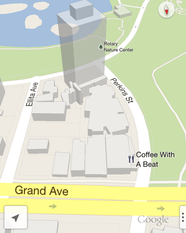
The translucent handling of the building is very good. It’s sketchy enough that you can recognize them and navigate without being distracted by their incompleteness.
Jan 5, 2013 7:53am
blog all oft-played tracks IV
This music:
- made its way to iTunes in 2012,
- and got listened to a lot.
I’ve made these for the past three years, lately. Also: everything as an .m3u playlist.
1. Goto80 and Raquel Meyers: Echidna, Moder Till Alla Monster

Do not miss the associated videos, 2sleep1.
2. Calvin-Harris: I Am Not Alone, Deadmau5 Remix

Sort of a stand-in for the entire remix collection by Deadmau5, on par with the Jesper Dahlbäck remixes. Also good is the Tiny Dancer remake.
3. VCMG: Spock

“VCMG” = Vince Clarke and Martin Gore, they of Depeche Mode making techno. Thanks Tomas for this recommendation.
4. Vitalic: Terminator Benelux

5. Operator: Midnight Star, Vocal LP Version

6. Orbital: The End Of The World

Orbital made a new album this year, and it’s good!
7. Yaz: Situation

8. Skinny Puppy: Assimilate, Live Amphi Festival 2010

This performance of 1984’s Assimilate has a harsher, more sawtooth wave timbre to it that I like very much.
9. Rihanna: SOS

10. Public Enemy: Harder Than You Think

This song crept onto the list in just the past few weeks, and it’s been on regular rotation in our house for weeks.
subscribe to ![]() this site.
|
contact Michal Migurski
this site.
|
contact Michal Migurski