tecznotes

Lake Merritt is the Lenna of cartography samples. Here’s one more from Ars Technica:

—Cyrus Farivar in Ars Technica, Hands-on with RunKeeper 3 for iPhone.

Usable line generalization for OSM roads and routes has been a hobby project of mine for several years now, since I argued for it at the first U.S. State of the Map conference in Atlanta, 2010. I’ve finally put the last piece of this project in place with the use of Hadoop to parallelize the geometry processing.

I’ve learned a lot about moving geographic data between Postgres and Hadoop. The result is available at Streets and Routes.

Matt Biddulph gave me a brief introduction to using Hadoop’s streaming utility, the summary of which was that it’s just a reasonably-smart manager of scripts that push text at each other:

The utility allows you to create and run Map/Reduce jobs with any executable or script as the mapper and/or the reducer. …both the mapper and the reducer are executables that read the input from stdin (line by line) and emit the output to stdout. The utility will create a Map/Reduce job, submit the job to an appropriate cluster, and monitor the progress of the job until it completes.

(MapReduce is Google’s 2004 data processing approach for big clusters)

I’d been building something like it myself, so it was a relief to dump everything and switch to Hadoop. Amazon’s Hadoop distribution, known as Elastic MapReduce, offers an additional layer of management, handling the setup and teardown of machines for you. Communication generally happens via S3, where you load your data and scripts and pick up your results. On the EC2 side, Amazon tends to use recent versions of Debian Linux 6.0, which means that all the nice geospatial packages you’d expect from apt are available.

Easy.

For this project, I’ve added Hadoop scripts directly to Skeletron, my line-generalization tool. There’s a mapper and a reducer. Everything speaks GeoJSON because it’s easy to parse in Python and use with Shapely. If you’re familiar with pipes in Unix, the entire process is exactly equivalent to this, spread out over many machines:

cat input | mapper | sort | reducer > output

The only tricky part is in the middle, because Hadoop’s sorting and distribution of the mapped output expects single lines of text with a tab-delimited key at the beginning. In Skeletron, I created a pair of functions that convert geographic features to text (base64-encoded Well-Known Binary) and back. Only the mapper’s input and reducer’s output need to speak and understand GeoJSON. Hadoop is pretty smart about the data it reads, as well. If you tell it to look in a directory on S3 for input and it finds a bunch of objects whose names end with “.bz2,” it will transparently decompress those for you before streaming them to a mapper.

So, the process of moving data from a PostGIS table created by osm2pgsql through Hadoop takes five steps:

1. Dump your geographic data into GeoJSON files.
2. Compress them and upload them to a directory on S3.
3. Run a MapReduce job that accepts and outputs GeoJSON data.
4. Wait.
5. Pick up resulting GeoJSON from another S3 directory.

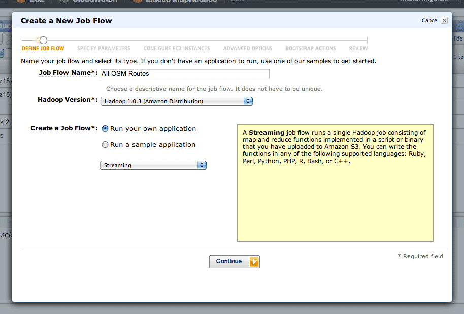
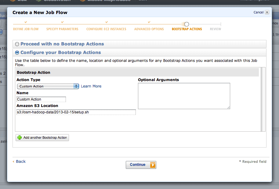
Running a MapReduce job is mostly a point-and-click affair.

After clicking the “Create New Job Flow” button from the AWS console, select the Streaming flow:

The second step is where you define your inputs, outputs, mappers and reducers:

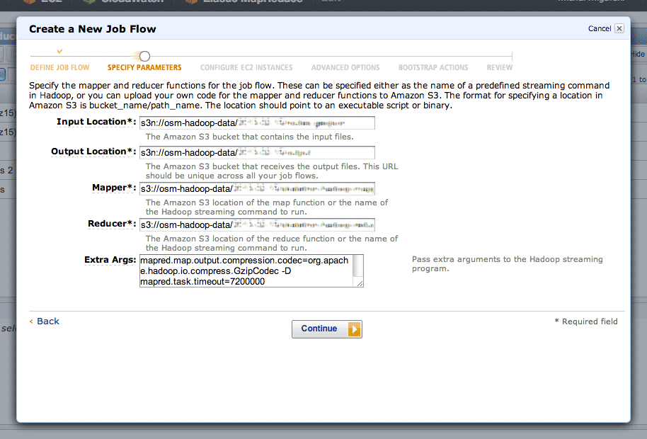
The “s3n:” protocol is used to refer to directories on S3, and the “osm-hadoop-data” part in the examples above is my bucket. For the mapper and reducer, I’ve uploaded the scripts directly from Skeletron so that EMR can find them.

The extra arguments I’ve used are:

• -D mapred.task.timeout=21600000 to give each map task six hours without Hadoop flagging it as failed. By default, Hadoop assumes that a task will take five minutes, but some of the more complex geometry tasks can take hours.
• -D mapred.compress.map.output=true to compress the data moving between the mappers and reducers, because it’s large and repetitive. The compression codec is given by -D mapred.map.output.compression.codec=org.apache.hadoop.io.compress.GzipCodec.
• -D mapred.output.compress=true to compress the output data sent to S3. The compression codec is given by -D mapred.output.compression.codec=org.apache.hadoop.io.compress.BZip2Codec.

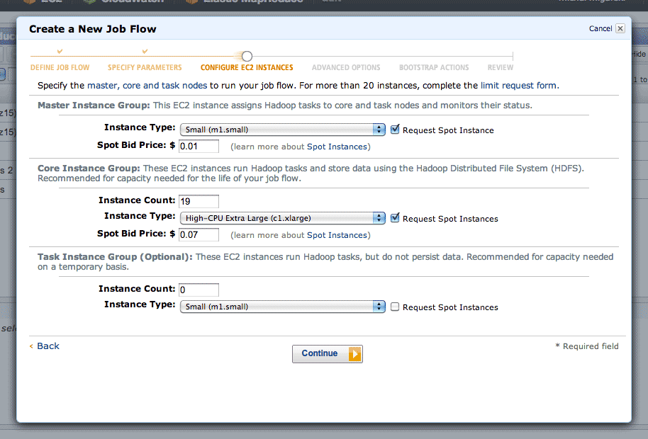
Step three is where you choose your EC2 machines. Amazon’s spot pricing is a smart thing to use here. I’ve typically seen prices on the order of $0.01 per CPU-hour, a huge savings on EC2’s normal pricing. Using the spot market will introduce some lag time to your job, since Amazon assumes you are a flexible cheapskate. I’ve typically experienced about ten minutes from creating a job to seeing it run.

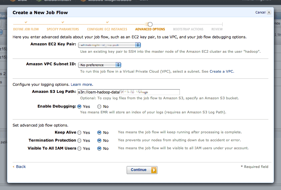
In step four, there are two interesting advanced options. Setting a log path will get you a directory full of detailed job logs, useful when something is mysteriously failing. Setting a key pair will allow you to SSH into your master instance, which runs a detailed Hadoop job tracker UI over HTTP on port 9100 (SSH tunnel in to see it in a browser). The tracker lets you dig into individual tasks or see an overall progress graph.

Step five is where you can define a setup script. This script is where you’ll do all of your per-machine preparation, such as downloading uniform data or installing additional packages.

For lengthy jobs, EMR’s graphs are a useful way to observe job flow progress. Your two most useful graphs are Average Map Tasks Running (top left), telling you how many mapper tasks are currently in progress, and Average Map Tasks Remaining (second from left on the top row), telling you how many mapper tasks have not yet started.

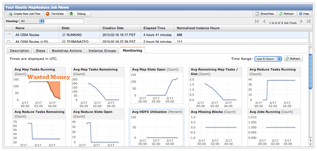
While the job is in progress, you’ll see the second graph progress downward toward zero, and the first graph pegged to the top and then progressing downward as well. The amount of time the first graph spends below the maximum represents wasted money, spent on CPU’s twiddling their thumbs waiting for straggler jobs to come in. This problem will be worse if you have more machines working on your job, leading to a very simple speed/cost tradeoff. If you want your job done fast, some of your machines won’t be doing much once the main crush is over. If you want your job done cheap, keep a smaller number of machines going to reduce the number of idle processors at the end.

I ran the same job twice with a different number of machines each time, and saw a cost of $4.90 for five instances over 17 hours vs. $9.40 for twenty instances over 7 hours. If you don’t need the results fast, save the five bucks and let it run overnight. If you don’t use spot pricing, this same job would have cost $40 slow or $78 fast.

To try all this yourself, I’ve set up a bucket with sample data from the OSM route relations job.

The end result is something I’m super happy about: a complete worldwide dataset of simplified roads and routes that’s suitable for high-quality labels and route shields.