tecznotes
Michal Migurski's notebook, listening post, and soapbox. Subscribe to ![]() this blog.
Check out the rest of my site as well.
this blog.
Check out the rest of my site as well.
Oct 25, 2015 7:25pm
projecting elevation data
I enjoy answering questions about geospatial techniques, and I’ve been trying to do it on this blog where others might benefit. I’ve done one about historical map projections and another about extracting point data from OSM.
I got an email from Djordje Spasic, a Serbian architect working on a project in Barcelona and trying to understand how to use elevation data in a modeling environment:
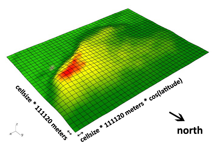
I am trying to create a digital terrain model of Barcelona, based on an .asc file, but in Rhino 5 application without the usage of NumPy. I attached the .asc file below. … I googled a bit and looks like both cell width and height should be 0.000833333333 decimal degrees. … There is one problem with this: I noticed that terrain model looks a bit stretched in east-west direction. Meaning, that the width of the cell is a bit too large. This got me thinking: is this due to significant latitude to which .asc file corresponds to (41.35 North)? I thought that maybe I could somehow not use equal cell width and height.
Djordje got in touch because of a hillshading script I had written, though I’ve also written a full library for tiling digital elevation models. Elevation data can be a pain to work with if you’re not familiar with either geographic projections or tools for working with raster data. Fortunately, GDAL does both if you know how to use it, and it comes built-in to QGIS, the desktop GIS application.
Based on the 0.00083 degree resolution, his data probably comes from the Shuttle Radar Topography Mission (SRTM) 3-arc-second data set, which has worldwide coverage at 1/1200° resolution. It’s also often known as the 90-meter dataset, because 1/1200° of latitude is a little over 90m on Earth.

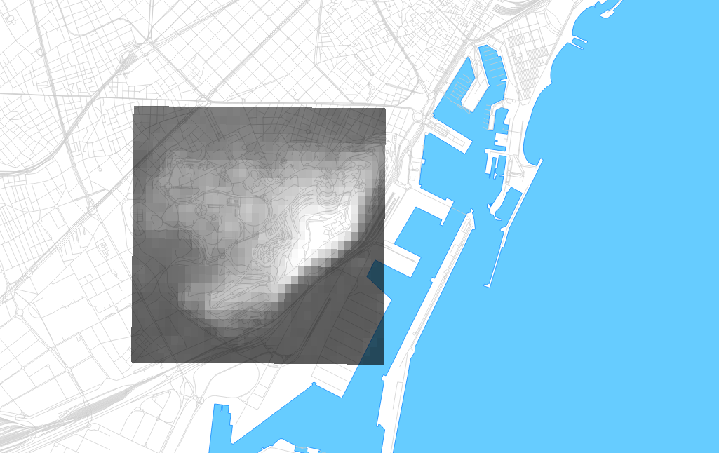
The tricky part is that degrees of longitude aren’t a consistent width on a spherical earth, and Djordje was getting confused about how to apply this dataset to an architectural model in a small, flat location. I pulled together some OpenStreetMap metro extract data for Barcelona, opened everything in QGIS, and set the projection to the UTM grid zone for Barcelona, 31N. UTM uses the conformal Mercator projection, and visualizing the layers immediately showed the stretching that Djordje described:
The cells are indeed about 90m North-South, but quite a bit less than that East-West due to the curvature of the earth’s surface. At the equator, they’d be square. At the poles, they’d be infinitely narrow. Here, the aspect ratio is about 1.2:1. Djordje’s first instinct was to simply scale the cells. That’d work for a small patch such as this, but would introduce distortions at larger sizes such as a whole city (approx. 27m of difference from southern to northern Barcelona over 1/4° of latitude).
It’s a relatively simple two-part operation to get the .asc file into a more correct form: first warp it, then translate it to a usable data format.
Warping on the command line is pretty easy:
gdalwarp -r cubic \
    -s_srs EPSG:4326 -t_srs EPSG:32631 \
    Barcelona_elevations.asc out.tif
Skipping the command line and warping in QGIS is also easy, using the menu command Raster ➤ Projections ➤ Warp.
EPSG:4326 is the spatial reference for unprojected degrees, and matches the source dataset of SRTM. EPSG:32631 is a spatial reference for Mercator meters in UTM zone 31N, a convenient choice for this location. I might also have chosen Google Maps Mercator if I didn’t care about meters specifically, or created a new projection centered on Barcelona if I wanted to be much more precise and have geographic North pointing exactly up. -r cubic uses a smoother interpolation function to generate new elevation values between the existing ones, similar to resizing a photo in Photoshop. The output file is a GeoTIFF, and looks like this in QGIS:
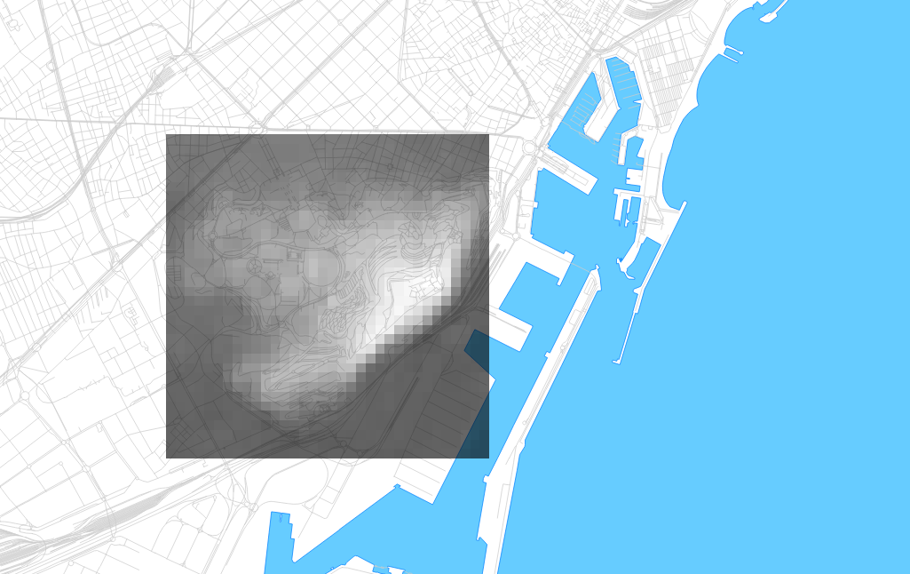
The individual pixels are now square, and at a known size of 78.9m on the ground. The grid is 34×34 instead of 34×29, after warping and interpolating new values to cover the same area. The visual differences between the two are minimal:

The format translation needs to be a second step, because GDAL and QGIS don’t know how to write to the ASCII grid format from the warp operation. I’m not sure why this is the case, but here is the second command:
gdal_translate -of AAIGrid out.tif out.ascTranslation is also available in QGIS as a menu command, under Raster ➤ Conversion ➤ Translate.
subscribe to ![]() this site.
|
contact Michal Migurski
this site.
|
contact Michal Migurski
Comments
Sorry, no new comments on old posts.